This page uses the following package. Make sure that you can load
them before trying to run the examples on this page. If you do not have
a package installed, run: install.packages("packagename"), or
if you see the version is out of date, run: update.packages().
Version info: Code for this page was tested in R version 3.0.1 (2013-05-16)
On: 2013-10-15
With: knitr 1.5; igraph 0.6.5-2
Plotting social network data can be easily done with the igraph package in R. This page will demonstrate some basic data management steps for social network data and provide the commands for creating a social network plot.
First, load the package igraph assuming it’s installed already:
require(igraph)
We will start with an adjacency table, mat25.txt.
x <- read.table("https://stats.idre.ucla.edu/stat/data/mat25.txt", header = FALSE)
head(x)
##   V1 V2 V3 V4 V5 V6 V7 V8 V9 V10 V11 V12 V13 V14 V15 V16 V17 V18 V19 V20
## 1  0  0  1  0  0  1  0  0  0   1   0   0   0   0   0   0   0   0   0   0
## 2  0  0  0  0  1  1  0  0  0   1   0   0   0   0   0   0   0   0   0   1
## 3  0  1  0  0  1  0  1  1  0   0   0   0   0   0   0   0   0   1   0   0
## 4  0  0  0  0  1  0  0  0  0   0   0   1   1   0   0   0   0   1   0   0
## 5  0  0  0  0  0  0  0  1  0   0   0   1   0   0   0   0   0   0   0   1
## 6  0  0  0  0  0  0  0  1  0   0   0   1   0   1   0   1   0   0   0   0
##   V21 V22 V23 V24 V25
## 1   0   1   0   1   0
## 2   1   0   0   0   0
## 3   0   0   0   0   0
## 4   0   0   0   1   0
## 5   1   0   0   0   1
## 6   1   0   0   0   0
In order for the igraph package to recognize this table as a network, we can
first convert it to a matrix. Then, if we wish to calculate graph-related
statistics on it (betweenness, closeness, degree), we can use the matrix to
create a graph object.
network <- as.matrix(x)
g1 <- graph.adjacency(network)
# compute betweenness
(b1 <- betweenness(g1, directed = FALSE))
##     V1     V2     V3     V4     V5     V6     V7     V8     V9    V10
## 12.510  4.109 10.409  4.920 11.346 12.489  1.835 14.577  6.052  6.901
##    V11    V12    V13    V14    V15    V16    V17    V18    V19    V20
##  4.176 10.283  7.496  9.331  2.147  4.066  1.069  4.217  4.420  9.077
##    V21    V22    V23    V24    V25
## 10.155  9.407  4.019 12.067  9.920
# compute closeness
(c1 <- closeness(g1, mode = "out"))
##      V1      V2      V3      V4      V5      V6      V7      V8      V9
## 0.01471 0.01408 0.01351 0.01408 0.01429 0.01408 0.01389 0.01408 0.01389
##     V10     V11     V12     V13     V14     V15     V16     V17     V18
## 0.01389 0.01408 0.01389 0.01429 0.01389 0.01408 0.01429 0.02041 0.01449
##     V19     V20     V21     V22     V23     V24     V25
## 0.01389 0.01449 0.01429 0.01429 0.01449 0.01449 0.01370
# compute degree
(d1 <- degree(g1, mode = "out"))
##  V1  V2  V3  V4  V5  V6  V7  V8  V9 V10 V11 V12 V13 V14 V15 V16 V17 V18
##   5   5   5   5   5   5   5   5   5   5   5   5   5   5   5   5   5   5
## V19 V20 V21 V22 V23 V24 V25
##   5   5   5   5   5   5   5
We have shown above how you can read an adjacency matrix as a table.
The igraph package also allows you to read in a dataset in which you list
the edges of a network. The file elist1.txt lists six edges:
1 2
1 3
1 4
3 5
4 6
6 4
We can read in this file as a graph, indicating that the format is an “edgelist”.
xlist <- read.graph("https://stats.idre.ucla.edu/stat/data/elist1.txt", format = "edgelist")
str(xlist)
## IGRAPH D--- 7 6 --
## + edges:
## [1] 2->3 2->4 2->5 4->6 5->7 7->5
Looking at the summary of our graph object, R believes our graph has 7 vertices although we only listed edges ranging from vertices 1 through 6. R makes a few assumptions unless otherwise specified:
- Vertices are indexed from zero and go through the highest numbered vertex in the edged list. You can specify that your graph contains more vertices than this, but not less.
- Edges are directed, going from the first vertex listed to the second.
We can amend our read.graph command to indicate that
our graph contains 8 vertices and that the edges are undirected. We
can then graph both and see the differences in nodes and edge
representations. Note that the plotting algorithm used does
not generate the same plot every time. In fact, it sometimes
generates plots in which vertices are crowded or overlapping or
edges are difficult to see. When this occurs, rerun the plot
command to get a new and likely better representation of your
network.
xlist.8un <- read.graph("https://stats.idre.ucla.edu/stat/data/elist1.txt", format = "edgelist",
    n = 8, directed = FALSE)
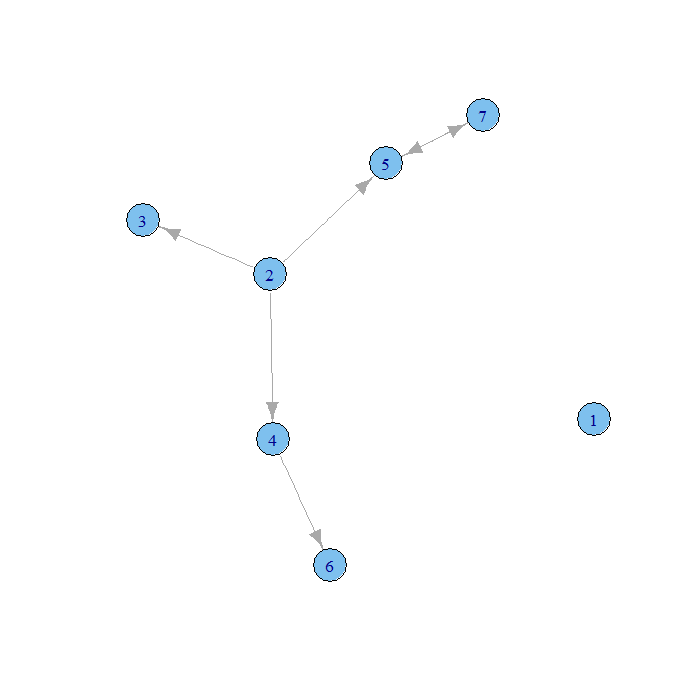
plot.igraph(xlist)

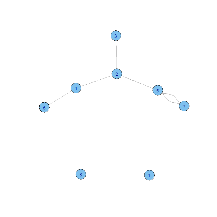
plot.igraph(xlist.8un)

Our first graph has an unconnected 0 vertex and arrows on the edges. Our second has unconnected 0 and 7 vertices and no arrows on the edges. We could also enter our data in a single vector of vertex indices where an edge connects the first and second, third and fourth, fifth and sixth entries and so on.
g2 <- graph(c(1, 2, 2, 3, 2, 4, 2, 5, 4, 6, 5, 7, 7, 5))
str(g2)
## IGRAPH D--- 7 7 --
## + edges:
## [1] 1->2 2->3 2->4 2->5 4->6 5->7 7->5
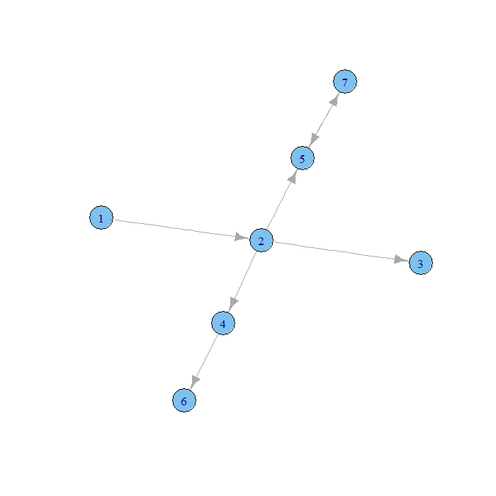
plot.igraph(g2)

For more information on the igraph package, see the igraph package R-project page or the igraph library page.
