
Attention
See this FAQ by Bauer that discusses the need to decompose within- and between-group effects when using this approach to ensure valid results (https://dbauer.web.unc.edu/wp-content/uploads/sites/7494/2015/08/Centering-in-111-Mediation.pdf).
FAQ starts here
Version info: Code for this page was tested in R version 3.1.1 (2014-07-10)

On: 2014-11-24

With: reshape2 1.4; lme4 1.1-7; Rcpp 0.11.2; Matrix 1.1-4; knitr 1.6
*Please note that the lme4 and nlme packages have changed since the creation of this page . The section of code covering the use of REmat from the lme4 package will no longer work with the current version of R (3.1.0). Also, the the method of estimation used in nlme has also changed. As such, the estimates presented here are slighly different than those received from the current version of R. We have plans to update the page as time permits.
Mediator variables are variables that sit between the independent variable and dependent variable and
mediate the effect of the IV on the DV. A model with one mediator is shown in the figure below.
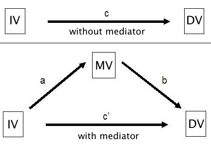
The idea, in mediation analysis, is that some of the effect of the predictor variable, the IV, is transmitted to the DV
through the mediator variable, the MV. And some of the effect of the IV passes directly to the
DV. That portion of of the effect of the IV that passes through the MV is the indirect
effect.
The FAQ page How can I perform mediation with multilevel data? (Method 1)
showed how to do multilevel mediation using an approach suggested by Krull & MacKinnon
(2001). This page will demonstrate an alternative approach given in the 2006 paper
by Bauer, Preacher & Gil. This approach combines the dependent variable and the
mediator into a single stacked response variable and runs one mixed model with indicator
variables for the DV and mediator to obtain
all of the values needed for the analysis.
We will begin by loading in a synthetic data set and reconfiguring it for our analysis.
All of the variables in this example (id the cluster ID, x the predictor
variable, m the mediator variable, and y the dependent variable) are at level 1
Here is how the first 16 observations look in the original dataset.
## read dataset in from internet
d <- read.csv("https://stats.idre.ucla.edu/stat/data/ml_sim.csv")

## view first 16 rows
d[1:16, ]
##    id       x       m      y
## 1   1  1.5451  0.1068  0.568
## 2   1  2.2753  2.1104  1.206
## 3   1  0.7867  0.0389 -0.261
## 4   1 -0.0619  0.4794 -0.759
## 5   1  0.1173  0.5908  0.519
## 6   1  1.4809  0.8909 -0.631
## 7   1  0.8928 -0.2277  0.152
## 8   1  0.9246  0.7292  0.235
## 9   2  1.0031 -0.3622 -1.151
## 10  2 -1.1914 -2.9658 -3.717
## 11  2 -1.8004 -3.6484 -4.470
## 12  2 -1.2585 -2.3043 -3.223
## 13  2 -0.4708 -1.4641 -2.661
## 14  2 -2.8150 -2.1196 -2.169
## 15  2 -0.2660 -0.3613 -2.173
## 16  2 -1.5617 -2.5556 -3.857
Let’s look at our data.
## summary information for each variable in the data frame
## exlcuding id by using -1 to remove first column
summary(d[, -1])
##        x               m               y
##  Min.   :-4.15   Min.   :-6.48   Min.   :-8.60
##  1st Qu.:-1.06   1st Qu.:-0.93   1st Qu.:-1.13
##  Median :-0.16   Median :-0.01   Median :-0.07
##  Mean   :-0.15   Mean   :-0.02   Mean   :-0.18
##  3rd Qu.: 0.75   3rd Qu.: 0.88   3rd Qu.: 0.86
##  Max.   : 3.87   Max.   : 5.01   Max.   : 5.92
## correlation matrix
cor(d[, -1])
##       x     m     y
## x 1.000 0.540 0.554
## m 0.540 1.000 0.759
## y 0.554 0.759 1.000
Let’s look at the three models of a mediation analysis beginning with the model with just the IV. We will use the lme4 package.
require(lme4)

## fit model and show summary
summary(m1 <- lmer(y ~ x + (1 + x | id), data = d))
## Linear mixed model fit by REML ['lmerMod']
## Formula: y ~ x + (1 + x | id)
##    Data: d
##
## REML criterion at convergence: 2435
##
## Scaled residuals:
##    Min     1Q Median     3Q    Max
## -3.316 -0.555  0.035  0.592  2.945
##
## Random effects:
##  Groups   Name        Variance Std.Dev. Corr
##  id       (Intercept) 0.747    0.864
##           x           0.217    0.466    -0.06
##  Residual             0.823    0.907
## Number of obs: 800, groups:  id, 100
##
## Fixed effects:
##             Estimate Std. Error t value
## (Intercept)  -0.0271     0.0960   -0.28
## x             0.6897     0.0586   11.76
##
## Correlation of Fixed Effects:
##   (Intr)
## x -0.018
Next, comes the model with the mediator predicted by the IV.
## fit model and show summary
summary(m2 <- lmer(m ~ x + (1 + x | id), data = d))
## Linear mixed model fit by REML ['lmerMod']
## Formula: m ~ x + (1 + x | id)
##    Data: d
##
## REML criterion at convergence: 2235
##
## Scaled residuals:
##    Min     1Q Median     3Q    Max
## -3.610 -0.617  0.022  0.616  2.914
##
## Random effects:
##  Groups   Name        Variance Std.Dev. Corr
##  id       (Intercept) 0.709    0.842
##           x           0.117    0.342    0.02
##  Residual             0.645    0.803
## Number of obs: 800, groups:  id, 100
##
## Fixed effects:
##             Estimate Std. Error t value
## (Intercept)   0.0952     0.0916    1.04
## x             0.6115     0.0464   13.17
##
## Correlation of Fixed Effects:
##   (Intr)
## x 0.049
Finally, the model with both the IV and mediator predicting the DV.
## fit model and show summary
summary(m3 <- lmer(y ~ m + x + (1 + m + x | id), data = d))
## Linear mixed model fit by REML ['lmerMod']
## Formula: y ~ m + x + (1 + m + x | id)
##    Data: d
##
## REML criterion at convergence: 2045
##
## Scaled residuals:
##    Min     1Q Median     3Q    Max
## -3.266 -0.585  0.017  0.604  2.336
##
## Random effects:
##  Groups   Name        Variance Std.Dev. Corr
##  id       (Intercept) 0.2615   0.511
##           m           0.1201   0.347    -0.03
##           x           0.0394   0.198    -0.31 -0.04
##  Residual             0.5077   0.713
## Number of obs: 800, groups:  id, 100
##
## Fixed effects:
##             Estimate Std. Error t value
## (Intercept)  -0.0937     0.0621   -1.51
## m             0.6251     0.0469   13.34
## x             0.2497     0.0387    6.44
##
## Correlation of Fixed Effects:
##   (Intr) m
## m -0.045
## x -0.084 -0.324
We see that the IV although still significant has been reduced. Now, we need to restructure the data to stack y on m for each row and create indicator variables for both the mediator and the dependent variables.
Here’s how we can do this using the reshape2 package.
require(reshape2)
d$fid <- 1:nrow(d)
stacked <- melt(d, id.vars = c("fid", "id", "x", "m"),
   measure.vars = c("y", "m"), value.name = "z")
stacked <- within(stacked, {
  sy <- as.integer(variable == "y")
  sm <- as.integer(variable == "m")
})

## show all data for id 1
stacked[stacked$id==1, ]
##     fid id       x       m variable       z sm sy
## 1     1  1  1.5451  0.1068        y  0.5678  0  1
## 2     2  1  2.2753  2.1104        y  1.2061  0  1
## 3     3  1  0.7867  0.0389        y -0.2613  0  1
## 4     4  1 -0.0619  0.4794        y -0.7590  0  1
## 5     5  1  0.1173  0.5908        y  0.5191  0  1
## 6     6  1  1.4809  0.8909        y -0.6311  0  1
## 7     7  1  0.8928 -0.2277        y  0.1521  0  1
## 8     8  1  0.9246  0.7292        y  0.2346  0  1
## 801   1  1  1.5451  0.1068        m  0.1068  1  0
## 802   2  1  2.2753  2.1104        m  2.1104  1  0
## 803   3  1  0.7867  0.0389        m  0.0389  1  0
## 804   4  1 -0.0619  0.4794        m  0.4794  1  0
## 805   5  1  0.1173  0.5908        m  0.5908  1  0
## 806   6  1  1.4809  0.8909        m  0.8909  1  0
## 807   7  1  0.8928 -0.2277        m -0.2277  1  0
## 808   8  1  0.9246  0.7292        m  0.7292  1  0
The new response variable is called z and has y stacked on m.
We named the indicators for the mediator and the DV sm and sy respectively,
to be consistent with Bauer et al (2006). We have also created a new m that
contains the value for the mediator from each of the original observations.
Notice that because we include the
sm and sy indicators in the model that we need to use the 0
to suppress the intercept.
## fit model
mm <- lmer(z ~ 0 + sm + sm:x + sy + sy:m + sy:x +
               (0 + sm + sm:x + sy + sy:m + sy:x | id) +
               (0 + sm | fid), data = stacked)
## view summary and save summary object to 'smm'
(smm <- summary(mm))
## Linear mixed model fit by REML ['lmerMod']
## Formula: z ~ 0 + sm + sm:x + sy + sy:m + sy:x + (0 + sm + sm:x + sy +
##     sy:m + sy:x | id) + (0 + sm | fid)
##    Data: stacked
##
## REML criterion at convergence: 4252
##
## Scaled residuals:
##    Min     1Q Median     3Q    Max
## -3.316 -0.572  0.028  0.582  2.617
##
## Random effects:
##  Groups   Name Variance Std.Dev. Corr
##  fid      sm   0.1378   0.371
##  id       sm   0.6794   0.824
##           sy   0.2703   0.520     0.13
##           sm:x 0.1205   0.347     0.06  0.07
##           sy:m 0.1119   0.334     0.03 -0.02  0.85
##           x:sy 0.0324   0.180    -0.04 -0.20 -0.34  0.09
##  Residual      0.5090   0.713
## Number of obs: 1600, groups:  fid, 800; id, 100
##
## Fixed effects:
##      Estimate Std. Error t value
## sm     0.0932     0.0894    1.04
## sy    -0.0969     0.0620   -1.56
## sm:x   0.6119     0.0465   13.16
## sy:m   0.6106     0.0455   13.41
## x:sy   0.2208     0.0372    5.93
##
## Correlation of Fixed Effects:
##      sm     sy     sm:x   sy:m
## sy    0.104
## sm:x  0.078  0.044
## sy:m  0.023 -0.040  0.465
## x:sy -0.017 -0.026 -0.114 -0.285
Note that the random slope sm by fid (the row id from the unstacked data set) is included to model the additional variance of the mediator variable, m. That is, this model should have two residual variances, one for the variable y and one for the variable m. That is actually accounted for. The residual variance for y is the overall model residual. The residual variance for m is the sum of the residual variance and the variance of the sm. The standard deviation is the square root of the sum of the variances. To do this, we will grab the random effects matrix from the REmat slot of the summary object, and drop the first two columns which are just names. Then we convert the matrix from character to numeric.
remat <- smm@REmat[, -c(1:2)]
## Error: trying to get slot "REmat" from an object (class
## "summary.merMod") that is not an S4 object
mode(remat) <- "numeric"
## Error: object 'remat' not found
## add rownames by collapsing group and name
rownames(remat) <- apply(smm@REmat[, 1:2], 1, paste, collapse = "")
## Error: trying to get slot "REmat" from an object (class
## "summary.merMod") that is not an S4 object
## variance and standard deviation of y
remat["Residual", c("Variance", "Std.Dev.")]
## Error: object 'remat' not found
## variance of m
sum(remat[c("fidsm", "Residual"), "Variance"])
## Error: object 'remat' not found
## standard deviation of m
sqrt(sum(remat[c("fidsm", "Residual"), "Variance"]))
## Error: object 'remat' not found
This can be accomplished more straightforwardly using the nlme package, which allows for residual variance structures. The varIdent function passed to the weights argument specifies constanct variance function separated by each level of variable, which is a factor indicator for y and m.
require(nlme)
## fit model
mm.alt <- lme(z ~ 0 + sm + sm:x + sy + sy:m + sy:x,
    data = stacked, random = ~0 + sm + sm:x + sy + sy:m +
        sy:x | id, weights = varIdent(form = ~1 | variable))

## view summary
summary(mm.alt)
## Linear mixed-effects model fit by REML
##  Data: stacked
##    AIC  BIC logLik
##   4296 4415  -2126
##
## Random effects:
##  Formula: ~0 + sm + sm:x + sy + sy:m + sy:x | id
##  Structure: General positive-definite, Log-Cholesky parametrization
##          StdDev Corr
## sm       0.824  sm     sy     sm:x   sy:m
## sy       0.520   0.133
## sm:x     0.347   0.063  0.066
## sy:m     0.334   0.034 -0.025  0.852
## x:sy     0.180  -0.045 -0.195 -0.344  0.090
## Residual 0.713
##
## Variance function:
##  Structure: Different standard deviations per stratum
##  Formula: ~1 | variable
##  Parameter estimates:
##    y    m
## 1.00 1.13
## Fixed effects: z ~ 0 + sm + sm:x + sy + sy:m + sy:x
##       Value Std.Error   DF t-value p-value
## sm    0.093    0.0894 1496    1.04   0.297
## sy   -0.097    0.0620 1496   -1.56   0.118
## sm:x  0.612    0.0465 1496   13.16   0.000
## sy:m  0.611    0.0455 1496   13.41   0.000
## x:sy  0.221    0.0372 1496    5.93   0.000
##  Correlation:
##      sm     sy     sm:x   sy:m
## sy    0.104
## sm:x  0.078  0.044
## sy:m  0.023 -0.040  0.465
## x:sy -0.017 -0.026 -0.114 -0.285
##
## Standardized Within-Group Residuals:
##     Min      Q1     Med      Q3     Max
## -3.6106 -0.6087  0.0297  0.6199  2.9497
##
## Number of Observations: 1600
## Number of Groups: 100
## detach nlme package since it masks aspects of lme4
detach("package:nlme")
This gives the residual standard deviation and the multiplier to obtain the residual standard deviation for y and m. Note that for y the multiplier is 1. That is, the residual standard deviation is for y. If we multiply the residual standard deviation by 1.127239, we get the residual standard deviation for m 0.804, which agrees with what we calculated from lmer.
We now have access to all of the information needed to compute the average indirect effect and average total effect and their standard errors using the equations given in Bauer, et. al. (2006). The average indirect effect formula is
$$ ind = ab + \sigma_{a_{j}b_{j}} \quad (EQ:A11)$$
$$Var(ind) = b^{2} \sigma^{2}_{\hat{a}} + a^{2} \sigma^{2}_{\hat{b}} +
\sigma^{2}_{\hat{a}}\sigma^{2}_{\hat{b}} + 2ab\sigma_{\hat{a},\hat{b}} +
(\sigma_{\hat{a},\hat{b}})^2 + \sigma^{2}_{\hat{\sigma}_{a_{j},b_{j}}} \quad (EQ:A14)
$$
average total effect
$$
tot = ab + \sigma_{a_{j}b_{j}} + c’ \quad (EQ:A15)
$$
$$
Var(ind) = b^{2}\sigma^{2}_{\hat{a}} + a^{2}\sigma^{2}_{\hat{b}} +
2ab\sigma_{\hat{a},\hat{b}} + 2b\sigma_{\hat{a},\hat{c}’} + 2a\sigma_{\hat{b},\hat{c}’} +
\sigma^{2}_{\hat{\sigma}_{a_{j},b_{j}}} + \sigma^{2}_{\hat{c}’} +
\sigma^{2}_{\hat{a}}\sigma^{2}_{hat{b}} + (\sigma_{hat{a},hat{b}})^2 \quad (EQ:A18)
$$
First, we can get the indirect effect by multiplying the fixed effects coefficients table and adding the covariance of their random effects. We can extract these using the functions fixef and VarCorr. lme helpfully provides the correlations among random effects. Unfortunately, this is a situation where we actually want the raw, unstandardized covariance. To get this will, we will have to back transform the correlation using the product of their standard deviations.
## view fixed effects estimates
fixef(mm)
##      sm      sy    sm:x    sy:m    x:sy
##  0.0932 -0.0969  0.6119  0.6106  0.2208
## product of 'a' and 'b' paths
(ab <- prod(fixef(mm)[c("sm:x", "sy:m")]))
## [1] 0.374
## covariance between random effects
(rcov <- VarCorr(mm)[["id"]]["sm:x", "sy:m"])
## [1] 0.099
## indirect effect
ab + rcov
## [1] 0.473
If we wanted to, we could also calculate the total effect, which is obtained by adding the direct effect of the predictor on the outcome to the indirect effect.
## total effect
ab + rcov + fixef(mm)["x:sy"]
##  x:sy
## 0.693
The standard error for the indirect and total effect are complicated. Future updates to this page may include them or alternatives such as bootstrapping or MCMC sampling.
References
- Bauer, D. J., Preacher, K. J. & Gil, K. M. (2006) Conceptualizing and testing random indirect
effects and moderated mediation in multilevel models: New procedures and recommendations.
Psychological Methods, 11(2), 142-163. - Krull, J. L. & MacKinnon, D. P. (2001) Multilevel modeling of individual and group level
mediated effects. Multivariate Behavioral Research, 36(2), 249-277. - The Stata page on the topic.