After you have finished your analysis in R, you may wish to save your data and/or graphs in a different format for use in other programs. We will start with a simple example in which we will take our sample data set (called hsb2) and save the data set in .csv format.
Saving a data set
There are a couple of different functions that you can use to write an R data set out to a different format. The function write.table is useful because it writes the data set out as a text file, which is easily read by most programs. We also used the option “row.names=F” to suppress the column of row numbers. The first ten lines of data are shown below and the first few lines from the exported text file are also shown below the command.
hsb2<-read.table("https://stats.idre.ucla.edu/stat/r/notes/hsb2.csv", sep=",", header=T)
attach(hsb2)
hsb2[1:10,]

    id female         race    ses schtyp     prog read write math science socst
1   70   male        white    low public  general   57    52   41      47    57
2  121 female        white middle public vocation   68    59   53      63    61
3   86   male        white   high public  general   44    33   54      58    31
4  141   male        white   high public vocation   63    44   47      53    56
5  172   male        white middle public academic   47    52   57      53    61
6  113   male        white middle public academic   44    52   51      63    61
7   50   male african-amer middle public  general   50    59   42      53    61
8   11   male     hispanic middle public academic   34    46   45      39    36
9   84   male        white middle public  general   63    57   54      58    51
10  48   male african-amer middle public academic   57    55   52      50    51
write.table(hsb2, "C:/temp/hsb2.txt",row.names=F) # change "C:/temp/" to the correct path for your computer
"id" "female" "race" "ses" "schtyp" "prog" "read" "write" "math" "science" "socst"
70 "male" "white" "low" "public" "general" 57 52 41 47 57
121 "female" "white" "middle" "public" "vocation" 68 59 53 63 61
86 "male" "white" "high" "public" "general" 44 33 54 58 31
141 "male" "white" "high" "public" "vocation" 63 44 47 53 56
172 "male" "white" "middle" "public" "academic" 47 52 57 53 61
While this works, you may not want strings enclosed in quotes. We can use the quote argument to prevent this.
write.table(hsb2, "C:/temp/hsb2a.txt",row.names=F,quote=FALSE)
id female race ses schtyp prog read write math science socst
70 male white low public general 57 52 41 47 57
121 female white middle public vocation 68 59 53 63 61
86 male white high public general 44 33 54 58 31
141 male white high public vocation 63 44 47 53 56
172 male white middle public academic 47 52 57 53 61
Saving a graph
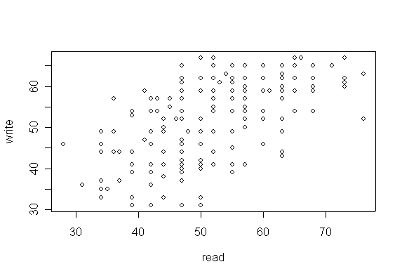
There are at least two ways that you can save a graph made in R into a different format (e.g., *.png). The first method involves opening a graph window, while the second method does not. We will create a simple scatter plot for use in our examples. Please note that this example will not work unless you have attached the data set, as we did above.
plot(read, write)
dev.print(device=postscript, "C:/temp/graph1.eps", onefile=FALSE, horizontal=FALSE)
In this example, the graph does not appear in a graph window in R. Rather, it just goes straight to the file specified.
postscript(file="C:/temp/graph2.eps", onefile=FALSE, horizontal=FALSE)
plot(read, write)
dev.off()
In this example, we save the graph as a .png file.
png("C:/temp/graph3.png")
hist(read)
dev.off()
In this example, we save the graph as a .pdf file.
pdf("D:/temp/graph4.pdf")
boxplot(write)
dev.off()
For more information on saving graphs in different formats, please refer to the help files for dev.print, dev.copy, and dev.copy2eps. You can also see our Library page on Graphing in R.

