When analyzing geospatial data, describing the spatial pattern of a measured
variable is of great importance. A common way of visualizing the spatial
autocorrelation of a variable is a variogram plot. This can be done in R.
There are several libraries with variogram capabilities. We will show how
to generate a variogram using the geoR library. To install, enter
install.packages("geoR") and then library(geoR) in R.
Let’s look at an example. Our dataset, ozone, contains ozone measurements from thirty-two locations in the Los Angeles area aggregated over one month. The dataset includes the station number (Station), the latitude and longitude of the station (Lat and Lon), and the average of the highest eight hour daily averages (Av8top). This data, and other spatial datasets, can be downloaded from the University of Illinois’s Spatial Analysis Lab. By generating a variogram, we will be able to look at the variance of the differences of Av8top among pairs of stations at different distances. We can look at a sample of our data and then a summary of the distances between the stations.
ozone<-read.table("https://stats.idre.ucla.edu/stat/r/faq/ozone.csv", sep=",", header=T)
head(ozone, n=10)

   Station   Av8top      Lat       Lon
1       60 7.225806 34.13583 -117.9236
2       69 5.899194 34.17611 -118.3153
3       72 4.052885 33.82361 -118.1875
4       74 7.181452 34.19944 -118.5347
5       75 6.076613 34.06694 -117.7514
6       84 3.157258 33.92917 -118.2097
7       85 5.201613 34.01500 -118.0597
8       87 4.717742 34.06722 -118.2264
9       88 6.532258 34.08333 -118.1069
10      89 7.540323 34.38750 -118.5347

dists <- dist(ozone[,3:4])
summary(dists)

   Min. 1st Qu.  Median    Mean 3rd Qu.    Max.
0.07267 0.39550 0.64660 0.73670 0.99190 2.39700
Next, we can calculate a variogram using the latitude and longitude of the stations. For this, we will use the variog command. We will indicate the distance intervals we wish to consider. Based on the summary of distances, we can look at 10 lag intervals of .15. To do this, we will first create a breaks vector of the endpoints of our intervals. To variog, we provide our coordinate variables and the “data”, the variable of interest. Then, we can look at the variog output that we will be plotting, the semi-variance, and the number of pairs counted in each interval. We want to check that our variogram is not calculating the semi-variance on small numbers of pairs.
breaks = seq(0, 1.5, l = 11)
v1
      lag semi-variance # of pairs
 [1,]   1      1.848505         21
 [2,]   2      1.841220         57
 [3,]   3      3.120452         74
 [4,]   4      4.375926         67
 [5,]   5      5.910725         71
 [6,]   6      7.097913         55
 [7,]   7      7.896033         44
 [8,]   8      6.571356         37
 [9,]   9      4.071090         23
[10,]  10      3.317602         16
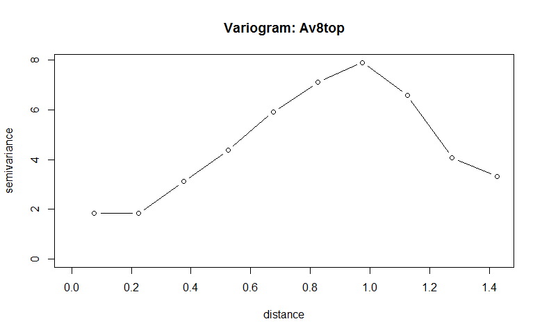
Now, we can plot the variogram:
plot(v1, type = "b", main = "Variogram: Av8top")
In the summary, we can see lag distances up to 10*.15 = 1.5, the number of pairs that are this far apart in the dataset, and the semi-variance. As we can see from the plot, the semi-variance increases until the lag distance exceeds 1.
Variograms in other packages:
References:
- Cressie, Noel. Statistics for Spatial Data. John Wiley & Sons, Inc.: New York, 1991.
