Predictive Mean Matching (PMM) is a semi-parametric imputation approach. It is similar to the regression method except that for each missing value, it fills in a value randomly from among the a observed donor values from an observation whose regression-predicted values are closest to the regression-predicted value for the missing value from the simulated regression model (Heitjan and Little 1991; Schenker and Taylor 1996).
The PMM method ensures that imputed values are plausible; it might be more appropriate than the regression method (which assumes a joint multivariate normal distribution) if the normality assumption is violated (Horton and Lipsitz 2001, p. 246).
This page uses the following packages. Make sure that you can load
them before trying to run the examples on this page. If you do not have
a package installed, run: install.packages("packagename"), or
if you see the version is out of date, run: update.packages().
library(mice)
library(VIM)
library(lattice)
library(ggplot2)
Version info: Code for this page was tested in R version 3.0.1 (2013-05-16)
On: 2013-11-08
With: ggplot2 0.9.3.1; VIM 4.0.0; colorspace 1.2-4; mice 2.18; nnet 7.3-7; MASS 7.3-29; lattice 0.20-23; knitr 1.5
Please note: The purpose of this page is to show how to use various data analysis commands associated with imputation using PMM. It does not cover all aspects of the research process which researchers are expected to do. In particular, it does not cover data cleaning and checking, verification of assumptions, model diagnostics and potential follow-up analyses. The page is based on a 2011 paper by Stef van Buuren and Karin Groothuis-Oudhoorn from the Jounal of Statsitical Software.
## Let us use the famous anscombe data and set a few to NA
anscombe <- within(anscombe, {
    y1[1:3] <- NA
    y4[3:5] <- NA
})
## view
anscombe
##    x1 x2 x3 x4    y1   y2    y3    y4
## 1  10 10 10  8    NA 9.14  7.46  6.58
## 2   8  8  8  8    NA 8.14  6.77  5.76
## 3  13 13 13  8    NA 8.74 12.74    NA
## 4   9  9  9  8  8.81 8.77  7.11    NA
## 5  11 11 11  8  8.33 9.26  7.81    NA
## 6  14 14 14  8  9.96 8.10  8.84  7.04
## 7   6  6  6  8  7.24 6.13  6.08  5.25
## 8   4  4  4 19  4.26 3.10  5.39 12.50
## 9  12 12 12  8 10.84 9.13  8.15  5.56
## 10  7  7  7  8  4.82 7.26  6.42  7.91
## 11  5  5  5  8  5.68 4.74  5.73  6.89
Missing Data Patterns
The Multiple Imputation by Chained Equations (MICE) package, not only allows for performing imputations but includes several functions for identifying the missing data pattern(s) present in a particular dataset.
## missing data patterns
md.pattern(anscombe)
##   x1 x2 x3 x4 y2 y3 y1 y4
## 6  1  1  1  1  1  1  1  1 0
## 2  1  1  1  1  1  1  0  1 1
## 2  1  1  1  1  1  1  1  0 1
## 1  1  1  1  1  1  1  0  0 2
##    0  0  0  0  0  0  3  3 6
The grid above represents the 4 missing data patterns present in our modified anscombe file. The first row represents the 6 observations that have complete information for all 8 variables. This is shown by having the value ‘1’ in each column representing non-missing information. The second column represents the 2 observations that are missing information only on the variable y1 .
## Number of observations per patterns for all pairs of variables
p <- md.pairs(anscombe)
p
## $rr
##    x1 x2 x3 x4 y1 y2 y3 y4
## x1 11 11 11 11  8 11 11  8
## x2 11 11 11 11  8 11 11  8
## x3 11 11 11 11  8 11 11  8
## x4 11 11 11 11  8 11 11  8
## y1  8  8  8  8  8  8  8  6
## y2 11 11 11 11  8 11 11  8
## y3 11 11 11 11  8 11 11  8
## y4  8  8  8  8  6  8  8  8
##
## $rm
##    x1 x2 x3 x4 y1 y2 y3 y4
## x1  0  0  0  0  3  0  0  3
## x2  0  0  0  0  3  0  0  3
## x3  0  0  0  0  3  0  0  3
## x4  0  0  0  0  3  0  0  3
## y1  0  0  0  0  0  0  0  2
## y2  0  0  0  0  3  0  0  3
## y3  0  0  0  0  3  0  0  3
## y4  0  0  0  0  2  0  0  0
##
## $mr
##    x1 x2 x3 x4 y1 y2 y3 y4
## x1  0  0  0  0  0  0  0  0
## x2  0  0  0  0  0  0  0  0
## x3  0  0  0  0  0  0  0  0
## x4  0  0  0  0  0  0  0  0
## y1  3  3  3  3  0  3  3  2
## y2  0  0  0  0  0  0  0  0
## y3  0  0  0  0  0  0  0  0
## y4  3  3  3  3  2  3  3  0
##
## $mm
##    x1 x2 x3 x4 y1 y2 y3 y4
## x1  0  0  0  0  0  0  0  0
## x2  0  0  0  0  0  0  0  0
## x3  0  0  0  0  0  0  0  0
## x4  0  0  0  0  0  0  0  0
## y1  0  0  0  0  3  0  0  1
## y2  0  0  0  0  0  0  0  0
## y3  0  0  0  0  0  0  0  0
## y4  0  0  0  0  1  0  0  3
The matrix (array) rr represents the number of observations where both pairs of values are observed. The matrix mm represents the exact opposite, these are the number of observations where both variables are missing values. The matrix rm shows the number of observations where the first variable’s value (i.e. the variable in the row) is observed and second (or column) variable is missing. The matrix mr is just the opposite of rm.
Missing Data Visualization
The VIM package in R can be used visualize missing data using several types of plots. We will demonstrate a few VIM package functions.
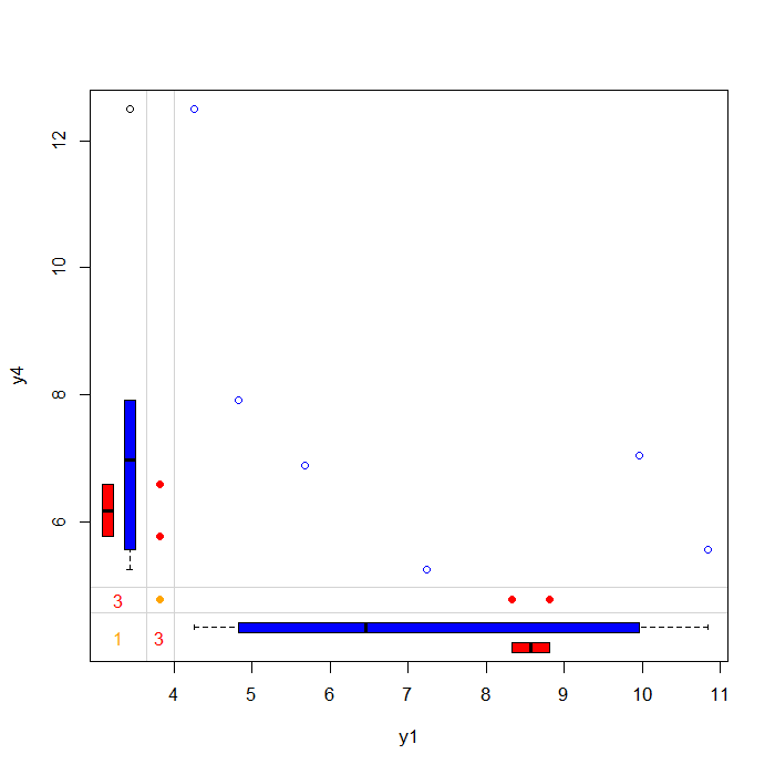
The marginplot function below will plot both the complete and incomplete observations for the variables specified. Here we will plot the available values for y1 and y4 .
## Margin plot of y1 and y4
marginplot(anscombe[c(5, 8)], col = c("blue", "red", "orange"))

The plot above allows you to examine the pattern and distribution of complete and incomplete observations. The blue dots represent individuals that have observed values for both y1 and y4 . The blue boxes located on the left and bottom margins are box plots of the non-missing values for each variable.
The red dots represent individuals that have missing values for either y1 but observed for y4 (left margin) or missing values for y4 but observed for y1 (bottom margin). The red boxes located on the left and bottom margins are box plots representing of the marginal distributions of these observed values.
Under the Missing Completely at Random (MCAR) assumption the red and blue box plots should be identical.
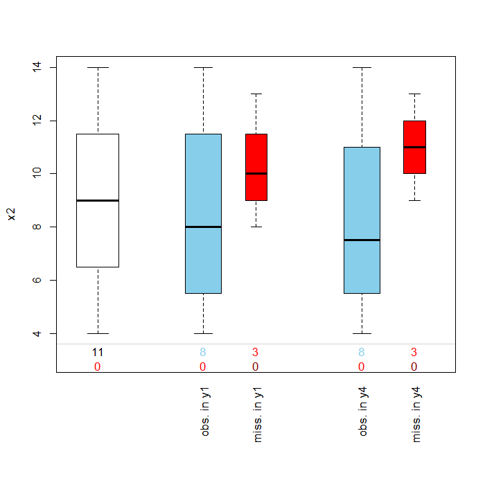
The pbox function below wil plot the marginal distribution of a variable within levels or categories of another variable. Here we obtain a plot of the distibution of the variable x2 by y1 and y4 . Pos=2 or position 2 in the anscombe file refers to the fact that x2 is in the second column of the data file.
## distributions of missing variable by another specified variable
pbox(anscombe, pos = 2)

In this cases as in the margins plot, the box plots are blue for observed values and red for missing values. This plot is useful is examining the Missing at Random (MAR) assumption that missingness is based on other observed variable(s) but not on the values of the missing variable(s) itself. Evidence supporting MAR over MCAR would be if the distribution of x2 for those observations with missing information for y1 or y4 were much higher or much lower than those of the non-missing observations. In the above graph, the boxplots appear to mostly overlap once again providing support for the assumption of MCAR.
Using MICE (Mulitple Imputation by Chained Equations)
The minimum information needed to use is the name of the data frame with missing values you would like to impute. The mice function will detect which variables is the data set have missing information. The default method of imputation in the MICE package is PMM and the default number of imputations is 5. If you would like to change the default number you can supply a second argument which we demonstrate below.
## by default it does 5 imputations for all missing values
imp1 <- mice(anscombe, m = 5)
##
##  iter imp variable
##   1   1  y1  y4
##   1   2  y1  y4
##   1   3  y1  y4
##   1   4  y1  y4
##   1   5  y1  y4
##   2   1  y1  y4
##   2   2  y1  y4
##   2   3  y1  y4
##   2   4  y1  y4
##   2   5  y1  y4
##   3   1  y1  y4
##   3   2  y1  y4
##   3   3  y1  y4
##   3   4  y1  y4
##   3   5  y1  y4
##   4   1  y1  y4
##   4   2  y1  y4
##   4   3  y1  y4
##   4   4  y1  y4
##   4   5  y1  y4
##   5   1  y1  y4
##   5   2  y1  y4
##   5   3  y1  y4
##   5   4  y1  y4
##   5   5  y1  y4
## Inspect the multiple imputed data set
imp1
## Multiply imputed data set
## Call:
## mice(data = anscombe, m = 5)
## Number of multiple imputations:  5
## Missing cells per column:
## x1 x2 x3 x4 y1 y2 y3 y4
##  0  0  0  0  3  0  0  3
## Imputation methods:
##    x1    x2    x3    x4    y1    y2    y3    y4
##    ""    ""    ""    "" "pmm"    ""    "" "pmm"
## VisitSequence:
## y1 y4
##  5  8
## PredictorMatrix:
##    x1 x2 x3 x4 y1 y2 y3 y4
## x1  0  0  0  0  0  0  0  0
## x2  0  0  0  0  0  0  0  0
## x3  0  0  0  0  0  0  0  0
## x4  0  0  0  0  0  0  0  0
## y1  1  0  0  1  0  1  1  1
## y2  0  0  0  0  0  0  0  0
## y3  0  0  0  0  0  0  0  0
## y4  1  0  0  1  1  1  1  0
## Random generator seed value:  NA
The output states that, as we requested, 5 imputed datasets were created. Our two variables with missing values were imputed using “pmm”. The predictor matrix tells us which variables in the dataset were used to produce predicted values for matching. For example, variables x1, x4 , y2-y4 were used to created predicted values for y1. We did not specify a seed value, so R chose one randomly; however, if you wanted to be able to reproduce your imputation you could set a seed for the random number generator.
Imputation Diagnostic Checks
As we mentioned earlier, one of the benefits to performing imputation using the method of PMM, is that we will get plausible values imputed. We can check the imputed values stored in each of the 5 imputed dataset stored in imp1.
imp1$imp$y1
##       1     2     3    4    5
## 1  8.81  7.24  8.81 8.81 7.24
## 2  8.33  8.33  7.24 7.24 8.33
## 3 10.84 10.84 10.84 9.96 9.96
The first three observation were missing information for y1. Above we can see what values were imputed for those observations in each of our 5 imputed datasets.
Now, before we can use our imputed datsets we need to combine them together with our original observed data. We can do this using a function in the mice package called complete . We will make our data long by stacking or appending our five imputed datasets and then we will use the inc=TRUE argument to specify we also want to append our observed original data.
Note: This “long” dataset is now in a format that can also be used for analysis in other statistical packages including SAS and Stata.
imp_tot2 <- complete(imp1, "long", inc = TRUE)
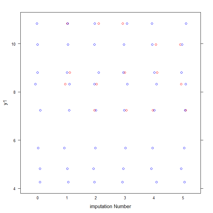
We can inspect the distributions of the original and imputed data using the stripplot function that is part of the lattice package.
## labels observed data in blue and imputed data in red for y1
col <- rep(c("blue", "red")[1 + as.numeric(is.na(imp1$data$y1))], 6)
## plots data for y1 by imputation
stripplot(y1 ~ .imp, data = imp_tot2, jit = TRUE, col = col, xlab = "imputation Number")

As you can see above, the blue dots represent the observed data values for y1 from the original anscombe file. The red dots represent the imputed values in each of our five imputed datasets.
Regression with imputed datasets
Now we are ready use are multiply imputed dataset in an analysis. We will demonstrate how do this, by running a linear regression model with y1 as the outcome and y4 and x1 as predictors.
## linear regression for each imputed data set - 5 regression are run
fitm <- with(imp1, lm(y1 ~ y4 + x1))
summary(fitm)
##
##  ## summary of imputation 1 :
##
## Call:
## lm(formula = y1 ~ y4 + x1)
##
## Residuals:
##    Min     1Q Median     3Q    Max
## -1.839 -0.353  0.126  0.506  0.817
##
## Coefficients:
##             Estimate Std. Error t value Pr(>|t|)
## (Intercept)   5.9529     1.6427    3.62  0.00675 **
## y4           -0.3650     0.1516   -2.41  0.04264 *
## x1            0.5133     0.0919    5.58  0.00052 ***
## ---
## Signif. codes:  0 '***' 0.001 '**' 0.01 '*' 0.05 '.' 0.1 ' ' 1
##
## Residual standard error: 0.86 on 8 degrees of freedom
## Multiple R-squared:  0.885,	Adjusted R-squared:  0.856
## F-statistic: 30.8 on 2 and 8 DF,  p-value: 0.000174
##
##
##  ## summary of imputation 2 :
##
## Call:
## lm(formula = y1 ~ y4 + x1)
##
## Residuals:
##    Min     1Q Median     3Q    Max
## -1.683 -0.561  0.402  0.702  0.992
##
## Coefficients:
##             Estimate Std. Error t value Pr(>|t|)
## (Intercept)    5.415      1.847    2.93   0.0189 *
## y4            -0.321      0.174   -1.85   0.1019
## x1             0.518      0.106    4.88   0.0012 **
## ---
## Signif. codes:  0 '***' 0.001 '**' 0.01 '*' 0.05 '.' 0.1 ' ' 1
##
## Residual standard error: 1.02 on 8 degrees of freedom
## Multiple R-squared:  0.839,	Adjusted R-squared:  0.798
## F-statistic: 20.8 on 2 and 8 DF,  p-value: 0.000677
##
##
##  ## summary of imputation 3 :
##
## Call:
## lm(formula = y1 ~ y4 + x1)
##
## Residuals:
##    Min     1Q Median     3Q    Max
## -1.691 -0.541  0.268  0.571  0.903
##
## Coefficients:
##             Estimate Std. Error t value Pr(>|t|)
## (Intercept)   5.0681     1.6223    3.12  0.01414 *
## y4           -0.2995     0.1519   -1.97  0.08417 .
## x1            0.5445     0.0929    5.86  0.00038 ***
## ---
## Signif. codes:  0 '***' 0.001 '**' 0.01 '*' 0.05 '.' 0.1 ' ' 1
##
## Residual standard error: 0.88 on 8 degrees of freedom
## Multiple R-squared:  0.881,	Adjusted R-squared:  0.851
## F-statistic: 29.5 on 2 and 8 DF,  p-value: 0.000204
##
##
##  ## summary of imputation 4 :
##
## Call:
## lm(formula = y1 ~ y4 + x1)
##
## Residuals:
##     Min      1Q  Median      3Q     Max
## -1.6816 -0.4355  0.0969  0.4771  1.0254
##
## Coefficients:
##             Estimate Std. Error t value Pr(>|t|)
## (Intercept)   5.3909     1.5415    3.50  0.00811 **
## y4           -0.3150     0.1455   -2.17  0.06226 .
## x1            0.5146     0.0877    5.87  0.00038 ***
## ---
## Signif. codes:  0 '***' 0.001 '**' 0.01 '*' 0.05 '.' 0.1 ' ' 1
##
## Residual standard error: 0.842 on 8 degrees of freedom
## Multiple R-squared:  0.88,	Adjusted R-squared:  0.85
## F-statistic: 29.4 on 2 and 8 DF,  p-value: 0.000205
##
##
##  ## summary of imputation 5 :
##
## Call:
## lm(formula = y1 ~ y4 + x1)
##
## Residuals:
##     Min      1Q  Median      3Q     Max
## -1.6262 -0.4712  0.0512  0.6208  1.3275
##
## Coefficients:
##             Estimate Std. Error t value Pr(>|t|)
## (Intercept)    5.996      1.861    3.22   0.0122 *
## y4            -0.343      0.169   -2.03   0.0769 .
## x1             0.452      0.108    4.18   0.0031 **
## ---
## Signif. codes:  0 '***' 0.001 '**' 0.01 '*' 0.05 '.' 0.1 ' ' 1
##
## Residual standard error: 0.967 on 8 degrees of freedom
## Multiple R-squared:  0.84,	Adjusted R-squared:   0.8
## F-statistic: 20.9 on 2 and 8 DF,  p-value: 0.000661
R will estimate our regression model separately for each imputed dataset, 1 though 5. We then need to summarize or pool those estimates to get one overall set of parameter estimates.
## pool coefficients and standard errors across all 5 regression models
pool(fitm)
## Call: pool(object = fitm)
##
## Pooled coefficients:
## (Intercept)          y4          x1
##       5.564      -0.329       0.509
##
## Fraction of information about the coefficients missing due to nonresponse:
## (Intercept)          y4          x1
##       0.267       0.238       0.331
## output parameter estimates
summary(pool(fitm))
##                est    se     t   df Pr(>|t|)  lo 95  hi 95 nmis   fmi
## (Intercept)  5.564 1.763  3.16 6.11  0.01917  1.270 9.8587   NA 0.267
## y4          -0.329 0.161 -2.04 6.34  0.08503 -0.718 0.0607    3 0.238
## x1           0.509 0.105  4.86 5.58  0.00344  0.248 0.7692    0 0.331
##             lambda
## (Intercept) 0.0614
## y4          0.0303
## x1          0.1272
Now we have one set of parameter estimates for our linear regression model
Additional Resources
You may also want to check out our FAQ page on how R handles missing data.
