Version info: Code for this page was tested in R Under development (unstable) (2012-07-05 r59734)
On: 2012-07-08
With: knitr 0.6.3
Please Note: The purpose of this page is to show how to use various data analysis commands. It does not cover all aspects of the research process which researchers are expected to do. In particular, it does not cover data cleaning and checking, verification of assumptions, model diagnostics and potential follow-up analyses.
Examples of multivariate random coefficient models
Example 1. A researcher has two outcomes he or she believes are predicted by the same set of predictors and would like to be able to directly test whether a predictor simultaneously significantly predicts both outcomes.
Description of the data
The data comes from an example in the Applied Longitudinal Data Analysis textbook. There are observations on a variety of measures over time nested within individuals. In addition to the time component, we are interested in two separate outcomes.
## read the data in
wages <- read.csv("https://stats.idre.ucla.edu/wp-content/uploads/2016/02/wages_pp-1.txt",head=TRUE)

## view the structure of the data
str(wages)
## 'data.frame':	6402 obs. of  15 variables:
##  $ id           : int  31 31 31 31 31 31 31 31 36 36 ...
##  $ lnw          : num  1.49 1.43 1.47 1.75 1.93 ...
##  $ exper        : num  0.015 0.715 1.734 2.773 3.927 ...
##  $ ged          : int  1 1 1 1 1 1 1 1 1 1 ...
##  $ postexp      : num  0.015 0.715 1.734 2.773 3.927 ...
##  $ black        : int  0 0 0 0 0 0 0 0 0 0 ...
##  $ hispanic     : int  1 1 1 1 1 1 1 1 0 0 ...
##  $ hgc          : int  8 8 8 8 8 8 8 8 9 9 ...
##  $ hgc.9        : int  -1 -1 -1 -1 -1 -1 -1 -1 0 0 ...
##  $ uerate       : num  3.21 3.21 3.21 3.29 2.9 ...
##  $ ue.7         : num  -3.79 -3.79 -3.79 -3.71 -4.11 ...
##  $ ue.centert1  : num  0 0 0 0.08 -0.32 ...
##  $ ue.mean      : num  3.21 3.21 3.21 3.21 3.21 ...
##  $ ue.person.cen: num  0 0 0 0.08 -0.32 ...
##  $ ue1          : num  3.21 3.21 3.21 3.21 3.21 ...
We will be working with the variables lnw and exper predicted from uerate all nested within id. First, we will calculate the mean of each variable by id and then view some summary information on these means by id. Like the minimum mean, mean mean, max mean.
with(wages, {
    ## find the mean of each variable by id
    tmp <- by(cbind(lnw, exper, uerate), id, colMeans, na.rm = TRUE)
    ## view summary informaiton the means by id for each variable
    summary(do.call("rbind", tmp))
})
##       lnw           exper          uerate
##  Min.   :1.06   Min.   :0.00   Min.   : 2.90
##  1st Qu.:1.67   1st Qu.:2.29   1st Qu.: 6.05
##  Median :1.84   Median :3.63   Median : 7.17
##  Mean   :1.88   Mean   :3.50   Mean   : 7.72
##  3rd Qu.:2.06   3rd Qu.:4.75   3rd Qu.: 8.78
##  Max.   :4.23   Max.   :8.31   Max.   :17.13
Now we can do the same thing, but instead of with means, do it with standard deviations. The summary information is now the mean standard deviation, the minimum standard deviation by id, etc.
with(wages, {
    ## find the variance of each variable by id
    tmp <- by(cbind(lnw, exper, uerate), id, function(x) sapply(x, sd, na.rm = TRUE))
    ## view summary informaiton the variances by id for each variable
    summary(do.call("rbind", tmp))
})
##       lnw          exper         uerate
##  Min.   :0.0   Min.   :0.0   Min.   :0.0
##  1st Qu.:0.2   1st Qu.:1.5   1st Qu.:1.3
##  Median :0.3   Median :2.3   Median :1.9
##  Mean   :0.3   Mean   :2.1   Mean   :2.0
##  3rd Qu.:0.4   3rd Qu.:2.8   3rd Qu.:2.6
##  Max.   :1.4   Max.   :4.6   Max.   :8.4
##  NA's   :38    NA's   :38    NA's   :38
The missing values (NAs) are caused by ids that do not have a calculable standard deviation. Either they are completely missing or there is no variability within those ids.
Analysis methods you might consider
- Multivariate random coefficient models, the focus of this page.
- Structural equation models with random effects
- Individual random coefficient models for each outcome. This will not produce multivariate results.
Multivariate random coefficient model analysis
Much like ANOVAs can be extended to MANOVAs, random coefficient models can be extended to have multiple outcome variables by stacking the outcomes on top of each other and coding which is which with dummy variables. To reshape the data, we will use the reshape2 package by Hadley Wickham. It provides a very easy interface for many cases of reshaping data from wide to long. In this case, we just want to stack the variables lnw and exper so those are the only names we pass to the measure.vars argument. The result is a new data set that is called swages for stacked wages. Note that we only keep the variables we will be using in this analysis. For the following analysis we will need the dplyr package.
require(dplyr)
require(reshape2)
swages <- melt(wages[, c("id", "uerate", "lnw", "exper")], measure.vars = c("lnw",
    "exper"))
swages <- within(swages, {
    Dl <- as.integer(variable == "lnw")
    De <- as.integer(variable == "exper")
})

## look at the structure of the new stacked data set
str(swages)
## 'data.frame':	12804 obs. of  6 variables:
##  $ id      : int  31 31 31 31 31 31 31 31 36 36 ...
##  $ uerate  : num  3.21 3.21 3.21 3.29 2.9 ...
##  $ variable: Factor w/ 2 levels "lnw","exper": 1 1 1 1 1 1 1 1 1 1 ...
##  $ value   : num  1.49 1.43 1.47 1.75 1.93 ...
##  $ De      : int  0 0 0 0 0 0 0 0 0 0 ...
##  $ Dl      : int  1 1 1 1 1 1 1 1 1 1 ...
## print the data for variables of interest for id 31
swages[swages$id == 31, ]
##      id uerate variable value De Dl
## 1    31   3.21      lnw 1.491  0  1
## 2    31   3.21      lnw 1.433  0  1
## 3    31   3.21      lnw 1.469  0  1
## 4    31   3.29      lnw 1.749  0  1
## 5    31   2.90      lnw 1.931  0  1
## 6    31   2.50      lnw 1.709  0  1
## 7    31   2.60      lnw 2.086  0  1
## 8    31   4.79      lnw 2.129  0  1
## 6403 31   3.21    exper 0.015  1  0
## 6404 31   3.21    exper 0.715  1  0
## 6405 31   3.21    exper 1.734  1  0
## 6406 31   3.29    exper 2.773  1  0
## 6407 31   2.90    exper 3.927  1  0
## 6408 31   2.50    exper 4.946  1  0
## 6409 31   2.60    exper 5.965  1  0
## 6410 31   4.79    exper 6.984  1  0
Dl and De are 0/1 dummy variables coding whether the outcome (now called value, the default name from the melt function) is the varialbe lnw or exper. id is now repeated many times and uerate is repeated twice, once for each outcome variable. To fit the model, we will use the nlme package. There is a new package appropriate for many types of random coefficient models, lme4 however it does not handle special residual covariance structures at the time of writing this page, so we use nlme instead. This multivariate model is special because the intercept is supressed (using the 0 notation) to allow for a separate intercept for each outcome indicate by the effect of the two dummy variables, De and Dl. Also notice that there are no “main effects” of the predictor, uerate. Instead, it is interacted with the dummy variables so that its slope can be different for the two outcomes. All of the terms are made random by id. Finally, a homogenous residual covariance structure is specified, but it is allowed to be different between the two outcome variables (so homogenous within outcome, heterogenous between).
Note that we specify special control arguments because the model did not converge in the default number of iterations, so they were increased.
require(nlme)
## fit the model, this may take some time
m <- lme(value ~ 0 + Dl + Dl:uerate + De + De:uerate, data = swages,
    random = ~0 + Dl + Dl:uerate + De + De:uerate | id, weights = varIdent(form = ~1 |
        variable), control = lmeControl(maxIter = 200, msMaxIter = 200, niterEM = 50,
        msMaxEval = 400))
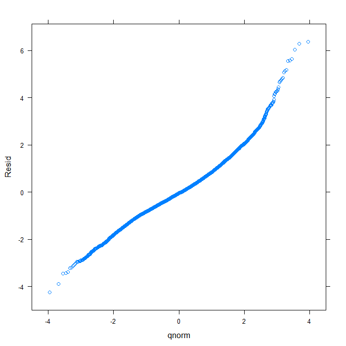
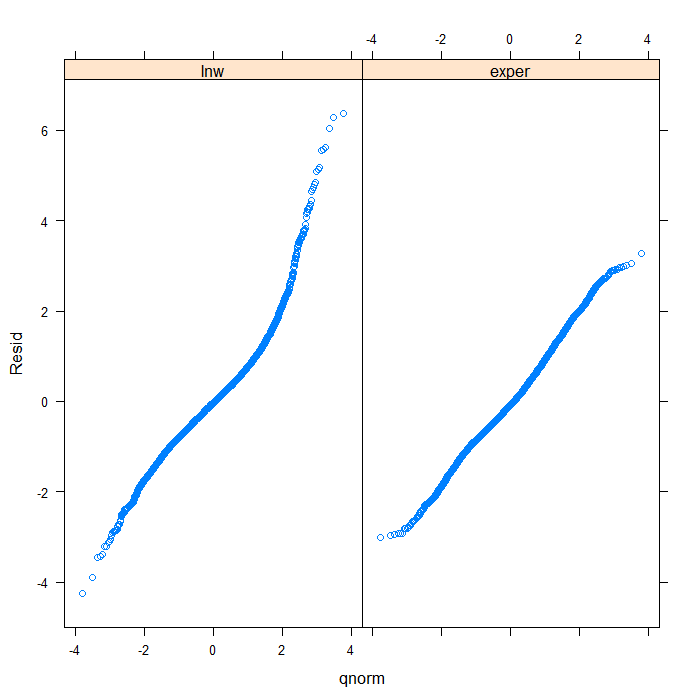
Before we look at coefficients and model parameters, let’s look at some diagnostic plots. First, we will look at the residuals against the fitted values. We will look at them overall, and broken down by outcome variable using the lattice package.
require(lattice)
## create data frame of residuals, fitted values, and variable
diagnos <- data.frame(Resid = resid(m, type = "normalized"), Fitted = fitted(m),
    Variable = swages$variable)

## overal QQ normal plot
qqmath(~Resid, data = diagnos, distribution = qnorm)
## separate by variable
qqmath(~Resid | Variable, data = diagnos, distribution = qnorm)
## we could add a line to indicate 'normal' with a bit more work
qqmath(~Resid | Variable, data = diagnos, distribution = qnorm, prepanel = prepanel.qqmathline,
    panel = function(x, ...) {
        panel.qqmathline(x, ...)
        panel.qqmath(x, ...)
    })
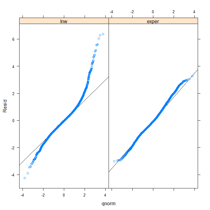
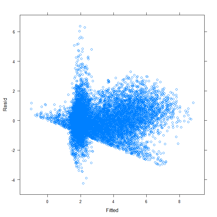
From the QQ plots of the residuals, it is pretty clear that they are not normally distributed and we might be concerned about that assumption. For the sake of demonstration, however, we will continue. Next, let’s look at the residuals plotted against the fitted values to check for things like heteroscedasticity.
## overall plot
xyplot(Resid ~ Fitted, data = diagnos)
## separate by variable
xyplot(Resid ~ Fitted | Variable, data = diagnos)
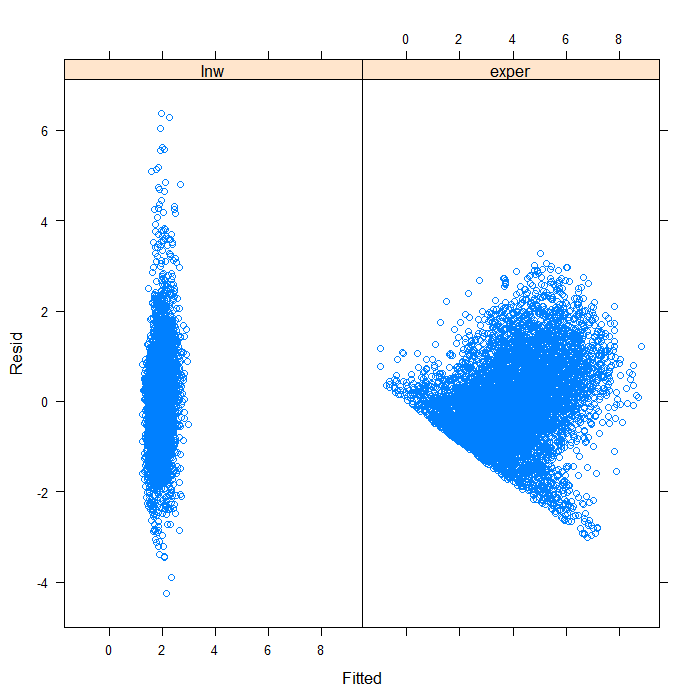
Separating by variable makes it look a bit better, though still far from ideal. We can see that the spread of predicted values is very different for the two variables. Hardly surprising given that they are not on the same scales. On that scale, it is difficult to see the real spread for lnw. We might examine the plot just for that variable.
xyplot(Resid ~ Fitted, data = subset(diagnos, Variable == "lnw"))
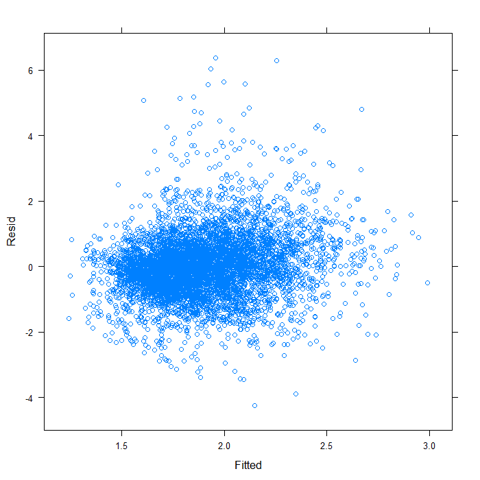
It does not seem too badly spread. Now we will look at QQ normal plots for each of the random effects. These are extracted from the model object using the ranef function.
rdiagnos <- ranef(m)
colnames(rdiagnos) <- c("lnw_int", "exper_int", "lnw_ue_slope", "exper_ue_slope")

## QQ normal for Dl random effect (random intercept)
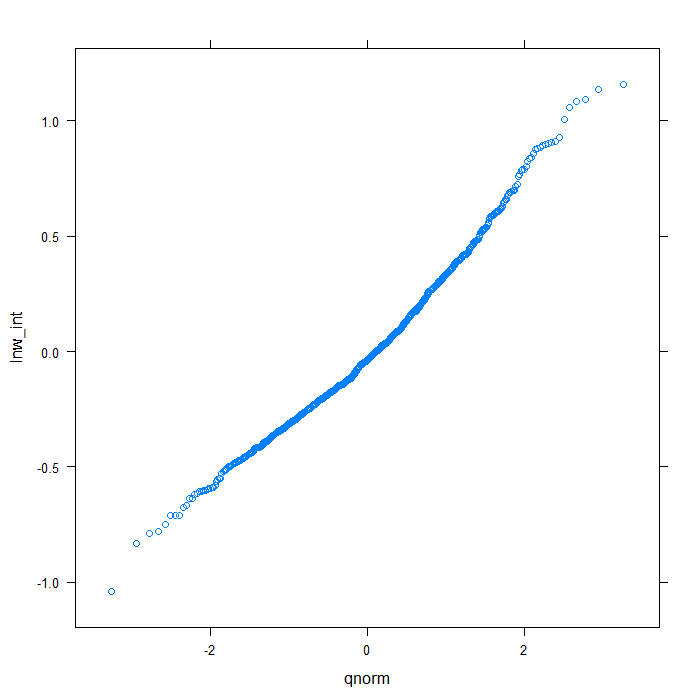
qqmath(~lnw_int, data = rdiagnos, distribution = qnorm)
## QQ normal for De random effect (random intercept)
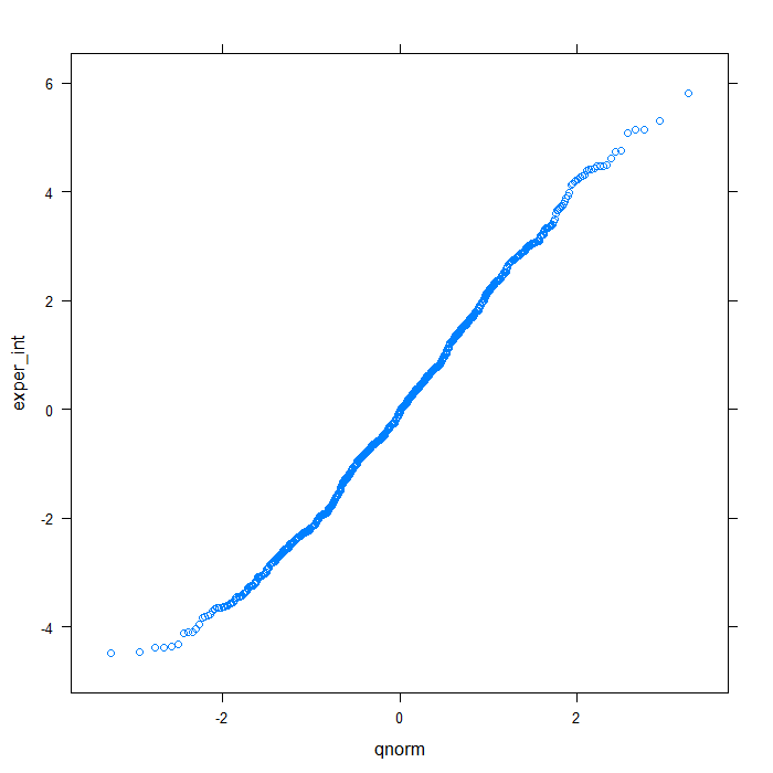
qqmath(~exper_int, data = rdiagnos, distribution = qnorm)
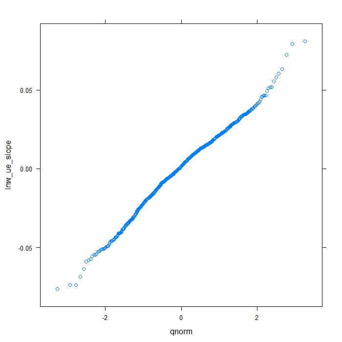
## QQ normal for uerate slope for lnw random effect
qqmath(~lnw_ue_slope, data = rdiagnos, distribution = qnorm)
## QQ normal for uerate slope for exper random effect
qqmath(~exper_ue_slope, data = rdiagnos, distribution = qnorm)
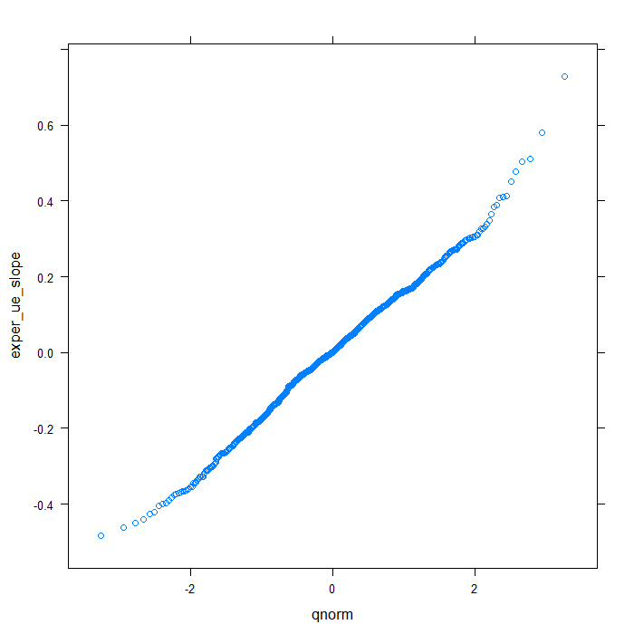
Happily, these plots all look very good. Finally, we will look at a summary of the model output.
## view a summary of the model
summary(m)
## Linear mixed-effects model fit by REML
##  Data: swages
##     AIC   BIC logLik
##   35213 35333 -17591
##
## Random effects:
##  Formula: ~0 + Dl + Dl:uerate + De + De:uerate | id
##  Structure: General positive-definite, Log-Cholesky parametrization
##           StdDev Corr
## Dl        0.423  Dl     De     Dl:urt
## De        2.700   0.557
## Dl:uerate 0.036  -0.829 -0.536
## uerate:De 0.268  -0.569 -0.852  0.739
## Residual  0.326
##
## Variance function:
##  Structure: Different standard deviations per stratum
##  Formula: ~1 | variable
##  Parameter estimates:
##   lnw exper
##  1.00  6.75
## Fixed effects: value ~ 0 + Dl + Dl:uerate + De + De:uerate
##           Value Std.Error    DF t-value p-value
## Dl         2.14    0.0204 11913   104.9       0
## De         6.86    0.1343 11913    51.1       0
## Dl:uerate -0.04    0.0022 11913   -16.9       0
## uerate:De -0.43    0.0155 11913   -27.5       0
##  Correlation:
##           Dl     De     Dl:urt
## De         0.361
## Dl:uerate -0.882 -0.330
## uerate:De -0.346 -0.899  0.402
##
## Standardized Within-Group Residuals:
##    Min     Q1    Med     Q3    Max
## -4.255 -0.579 -0.048  0.520  6.377
##
## Number of Observations: 12804
## Number of Groups: 888
It gives us a lot of information. Not immediately obvious is that the residual standard deviation (square root of the residual variance) is for the lne variable. To get the value for the exper variable, multiple the residual by 6.74675. That is how much bigger the residual variance for the exper variable was than for the lnw variable, which equals 2.197.
Things to consider
These models can easily become quite complex and may run into convergence problems as well as being slow. It is easy to misspeficy the random effects and covariance structure. There is some literature on this, but it is not a very common technique. It may require careful explanation to your readers.
See also
Structural Equation Modelling programs like Mplus or EQS that can fit SEM models with random effects (multilevel SEM).
References
Multilevel Analysis: Techniques and Applications by Joop Hox has a chapter that describes these kinds of models. Most other multilevel textbooks seem to maybe have small sections where it is described but not extensive detail.
