Random Coefficient Poisson Models

Version info: Code for this page was tested in R Under development (unstable) (2012-07-05 r59734) On: 2012-07-08 With: knitr 0.6.3

Please Note: The purpose of this page is to show how to use various data analysis commands. It does not cover all aspects of the research process which researchers are expected to do. In particular, it does not cover data cleaning and checking, verification of assumptions, model diagnostics and potential follow-up analyses.

Examples of random coefficient poisson models

Poisson models are useful for count data. Examples could include number of traffic tickets an individual receives in a year, number of tumor sites in cancer patients, or number of awards received by students. In each of these cases, we might expect most people to have very few, with a relatively small number of individuals having higher numbers.

Background on the Poisson distribution

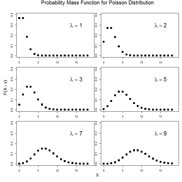
Unlike the familiar Gaussian distribution which has two parameters (mathcal{N}(mu, sigma^{2})), the Poisson distribution is described by a single parameter, (lambda) that is both the mean and variance. That is, (lambda = E(x)) and (lambda = Var(x) = E(x^{2}) – E(x)^{2}). In many ways, this can be a strong assumption. In some cases, use of the negative binomial distribution which estimates a second scale parameter to allow for overdispersion. Here is what the Poisson distribution looks like for different values of (lambda).

par(mfrow = c(3, 2), mar = c(1, 1, 2, 1), oma = c(4, 4, 2, 0))
for (i in c(1, 2, 3, 5, 7, 9)) {
    curve(dpois(x, lambda = i), from = 0, to = 18, n = 19, type = "p", pch = 15,
        cex = 1.5, xlim = c(0, 19), ylim = c(0, 0.4), xlab = "", ylab = "")
    text(x = 15, y = 0.3, substitute(lambda == x, list(x = i)), cex = 2)
}
mtext("Probability Mass Function for Poisson Distribution", line = 0.5,
    outer = TRUE, cex = 1.2)
mtext(expression(P(X == x)), side = 2, line = 1.5, outer = TRUE)
mtext("X", side = 1, line = 1.5, outer = TRUE)

Without random coefficients, the standard Poisson model is:

\begin{equation} \log E(y_{i}) = \alpha + X’_{i} \beta \end{equation}

The log link is the canonical link function for the Poisson distribution, and the expected value of the response is modeled.

With random coefficients, for example a random intercept, the model becomes:

\begin{equation} \log E(y_{ij}|u_{j}) = \alpha + X’_{ij} \beta + u_{j} \end{equation}

Where \(y_{ij}\) is the observation for individual (i) in group (j) and \(u_{j}\) is the random effect for group (j). Thus the two distributions are:

\begin{equation} y \sim Pois(\lambda) \end{equation}

and

\begin{equation} u \sim N(0, \sigma^{2}) \end{equation}

The random coefficient model is conditional on the random effect. To show what this means, consider a simple model:

\begin{equation} \log E(y_{ij}|u_{j}) = -.5 + .3x_{ij} + u_{j} \end{equation}

In the original units, this becomes:

\begin{equation} E(y_{ij}|u_{j}) = \exp(-.5 + .3x_{ij} + u_{j}) \end{equation}

Now look what happens when we graph the estimated change for a 1 unit change in x for values of the random variable (u) ranging from 0 to 4 by increments of .5.

par(mfrow=c(1,1))
f <- function(x_ij, u_j) {

    exp(-0.5 + x_ij * 0.3 + u_j)
}
for (i in seq(0, 4, 0.5)) {
    curve(f(x, u_j = i), from = 0, to = 1, n = 200, add = i > 0, ylim = c(0,
        45), ylab = "")
}
title(ylab = bquote(E(Y ~ l ~ x[ij], u[j])), main = "Effect of x for different random effects")

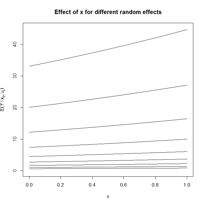
Clearly, on the scale of the original units, a 1 unit increase in x has different effects depending on the value of u, hence the conditionalness of the model. Population “average” effects can be obtained by integrating out the random effect or by fitting a marginal model such as using GEEs.

Although the outcome is assumed to have a Poisson distribution, the random effect (in the above example, u) is typically assumed to have a Gaussian distribution.

Description of the data

The example data we use comes from a sample of the high school and beyond data set, with a made up variable, number of awards a student receives, awards. Our main predictor will be sex, female, and students are clustered (grouped) within schools, cid. First, we will load all the packages required for these examples.

## load foreign package to read Stata data files
require(foreign)

## ggplot2 package for graphs
require(ggplot2)

You need to install the glmmADMB() package via instructions given in http://glmmadmb.r-forge.r-project.org/. Note that if you are not able to install the glmmADMB() package you may need to use Rtools and compile from source, use Linux, or ask the authors of the package for more information.

install.packages("R2admb")

install.packages("glmmADMB",
                  repos="http://glmmadmb.r-forge.r-project.org/repos",
                  type="source")

require(glmmADMB)

## load lme4 package
require(lme4)

## read in data
dat <- read.dta("https://stats.idre.ucla.edu/stat/data/hsbdemo.dta")
dat$cid <- factor(dat$cid)

## look at the first few rows of the dataset
head(dat)

   id female    ses schtyp     prog read write math science socst       honors awards cid
1  45 female    low public vocation   34    35   41      29    26 not enrolled      0   1
2 108   male middle public  general   34    33   41      36    36 not enrolled      0   1
3  15   male   high public vocation   39    39   44      26    42 not enrolled      0   1
4  67   male    low public vocation   37    37   42      33    32 not enrolled      0   1
5 153   male middle public vocation   39    31   40      39    51 not enrolled      0   1
6  51 female   high public  general   42    36   42      31    39 not enrolled      0   1

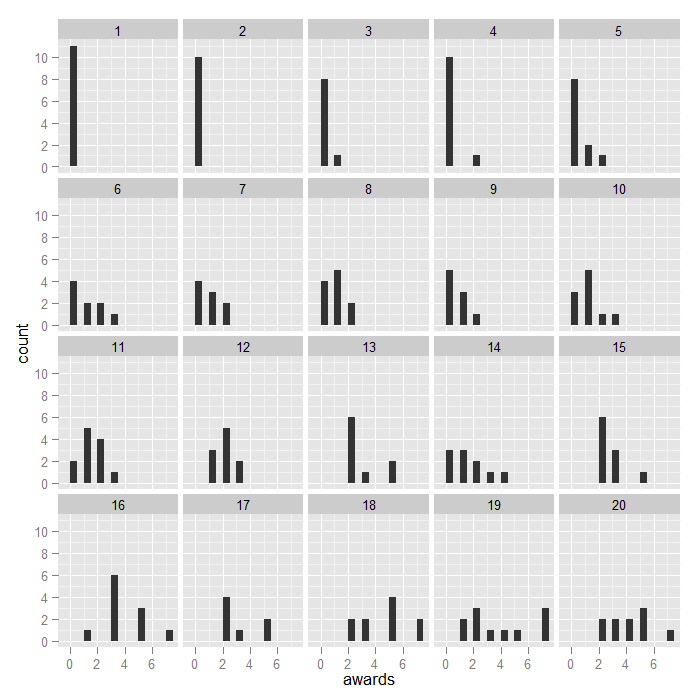
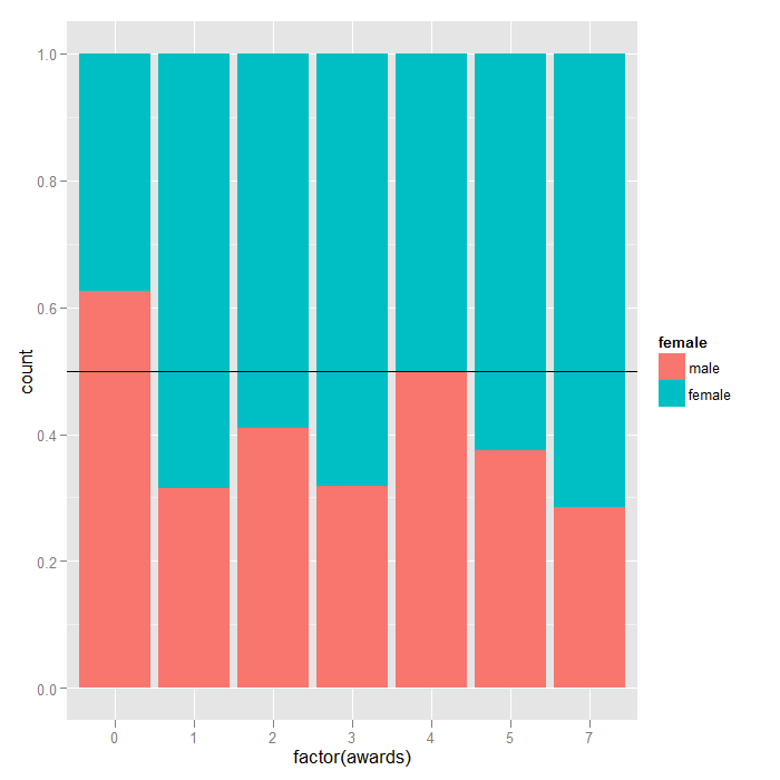
We can get a sense of the distributions in the data using the ggplot2 package. The first plot is just histograms of number of awards for every cid. The second is a filled density plot. The density sums to 1 and the fill shows the distribution of female at every level of awards. If the distribution of female is equal across all awards, they would fall on the horizontal line.

## awards by school

ggplot(dat, aes(awards)) + geom_histogram(binwidth = 0.5) + facet_wrap(~cid)

## density of awards by sex, line at .5 is the null of no sex differences
## in number of awards
ggplot(dat, aes(factor(awards))) + geom_bar(aes(fill = female), position = "fill") + geom_hline(yintercept = 0.5)

Analysis methods you might consider

Random coefficient poisson models, the focus of this page.
Poisson regression with robust standard errors

Random coefficient poisson model analysis

Because generalized linear mixed models (GLMMs) such as random coefficient poisson models are rather difficult to fit, there tends to be some variability in parameter estimates between different programs. We will demonstrate the use of two packages in R that are able to fit these models, lme4 and glmmADMB.

## fit a random intercept only model using the Laplace approximation
## (equivalent to 1 point evaluated per axis in Gauss-Hermite
## approximation)
m1a <- glmer(awards ~ 1 + (1 | cid), data = dat, family = poisson(link = "log"))
## fit a random intercept only model using 100 points per axis in the
## adaptive Gauss-Hermite approximation of the log likelihood more points
## improves accuracy but will take longer
m1b <- glmer(awards ~ 1 + (1 | cid), data = dat, family = poisson(link = "log"), nAGQ = 100)

## compare (only slightly different)
rbind(m1a = coef(summary(m1a)), m1b = coef(summary(m1b)))

##              Estimate Std. Error  z value Pr(>|z|)
## (Intercept) -0.008853     0.2826 -0.03133   0.9750
## (Intercept) -0.009280     0.2834 -0.03275   0.9739

## view summary output from the more accurate model
summary(m1b)

Generalized linear mixed model fit by maximum likelihood (Adaptive Gauss-Hermite Quadrature, nAGQ =
  100) [glmerMod]
 Family: poisson  ( log )
Formula: awards ~ 1 + (1 | cid)
   Data: dat

     AIC      BIC   logLik deviance df.resid 
   228.6    235.2   -112.3    224.6      198 

Scaled residuals: 
    Min      1Q  Median      3Q     Max 
-1.3857 -0.5260 -0.3383  0.3379  3.3769 

Random effects:
 Groups Name        Variance Std.Dev.
 cid    (Intercept) 1.458    1.207   
Number of obs: 200, groups:  cid, 20

Fixed effects:
             Estimate Std. Error z value Pr(>|z|)
(Intercept) -0.009575   0.290294  -0.033    0.974

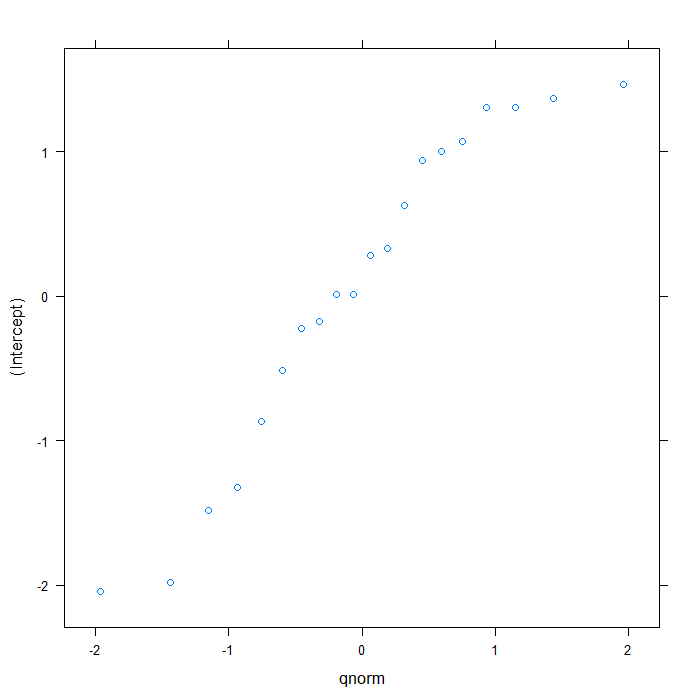
We can visually inspect the random effects with a Q-Q plot or a caterpillar plot

## QQ plot
plot(ranef(m1b))

## $cid

## Caterpillar plot
lattice::dotplot(ranef(m1b, postVar = TRUE))

## $cid

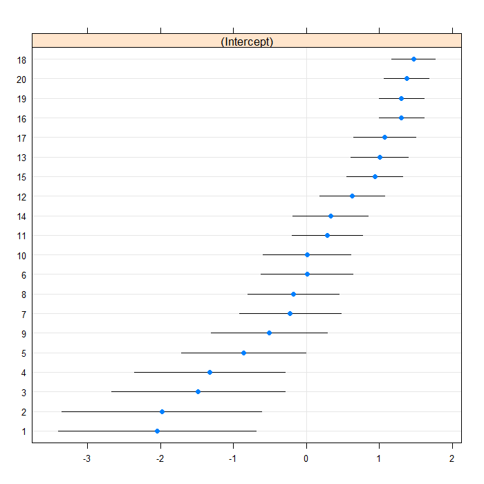
The estimate for the intercept is essentially 0, although the random effects variance indicates that there is some variability in the intercepts between schools. Now we will add in female as an explanatory variable.

m2 <- glmer(awards ~ 1 + female + (1 | cid), data = dat, family = poisson(link = "log"), nAGQ = 100)
summary(m2)

Generalized linear mixed model fit by maximum likelihood (Adaptive Gauss-Hermite Quadrature, nAGQ =
  100) [glmerMod]
 Family: poisson  ( log )
Formula: awards ~ 1 + female + (1 | cid)
   Data: dat

     AIC      BIC   logLik deviance df.resid 
   221.1    231.0   -107.6    215.1      197 

Scaled residuals: 
    Min      1Q  Median      3Q     Max 
-1.5312 -0.5919 -0.3304  0.2047  2.8806 

Random effects:
 Groups Name        Variance Std.Dev.
 cid    (Intercept) 1.431    1.196   
Number of obs: 200, groups:  cid, 20

Fixed effects:
             Estimate Std. Error z value Pr(>|z|)   
(Intercept)   -0.2229     0.2975  -0.749  0.45370   
femalefemale   0.3632     0.1193   3.044  0.00234 **
---
Signif. codes:  0 ‘***’ 0.001 ‘**’ 0.01 ‘*’ 0.05 ‘.’ 0.1 ‘ ’ 1

Correlation of Fixed Effects:
            (Intr)
femalefemal -0.252

There appears to be a fairly strong effect of females such that females tend to get more awards than males. Now we will fit the same models using the glmmADMB package

## random intercept only model
library(glmmADMB)

m.alt1 <- glmmadmb(awards ~ 1 + (1 | cid), data = dat, family = "poisson", link = "log")
m.alt2 <- glmmadmb(awards ~ 1 + female + (1 | cid), data = dat, family = "poisson", link = "log")

summary(m.alt1)

Call:
glmmadmb(formula = awards ~ 1 + (1 | cid), data = dat, family = "poisson", 
    link = "log")

AIC: 575.1 

Coefficients:
            Estimate Std. Error z value Pr(>|z|)
(Intercept) -0.00881    0.28902   -0.03     0.98

Number of observations: total=200, cid=20 
Random effect variance(s):
Group=cid
            Variance StdDev
(Intercept)    1.443  1.201


Log-likelihood: -285.528

summary(m.alt2)

Call:
glmmadmb(formula = awards ~ 1 + female + (1 | cid), data = dat, 
 family = "poisson", link = "log")

AIC: 567.5 

Coefficients:
 Estimate Std. Error z value Pr(>|z|) 
(Intercept) -0.222 0.296 -0.75 0.4534 
femalefemale 0.363 0.119 3.04 0.0023 **
---
Signif. codes: 0 ‘***’ 0.001 ‘**’ 0.01 ‘*’ 0.05 ‘.’ 0.1 ‘ ’ 1

Number of observations: total=200, cid=20 
Random effect variance(s):
Group=cid
 Variance StdDev
(Intercept) 1.417 1.19


Log-likelihood: -280.769

The results from glmmadmb match closely with those from glmer.

Things to consider

There have been reports (e.g., Zhang et al, 2009) of inconsistency and substantial alpha inflation between different statistical packages and estimation techniques (e.g., using penalized quasi-likelihood, Laplace approximation, Gauss-Hermite quadrature).

SAS

The dataset can be downloaded from here: hsbdemo

data dat;
  set "c:\temp\hsbdemo.sas7bdat";
run;

proc sort data=dat;
  by cid descending female;
run;

PROC GLIMMIX data = dat method=LAPLACE noclprint;
  class cid;
  model awards = / solution dist=poisson;
  random intercept / subject=cid;
run;

PROC GLIMMIX data = dat method=QUAD(QPOINTS = 100) noclprint;
  class cid;
  model awards = / solution dist=poisson;
  random intercept / subject=cid;
run;

PROC GLIMMIX data = dat method=LAPLACE noclprint order = data;
  class female cid;
  model awards = female / solution dist=poisson;
  random intercept / subject=cid;
run;

PROC GLIMMIX data = dat method=QUAD(QPOINTS = 100) noclprint order = data;
  class female cid;
  model awards = female / solution dist=poisson;
  random intercept / subject=cid;
run;

/*We can also manually parameterize the model in NLMIXED */
PROC NLMIXED data = dat METHOD=GAUSS QPOINTS=100;
  eta = alpha + u;
  lambda = exp(eta);
  model awards ~ poisson(lambda);
  random u ~ normal(0, exp(2*log_sigma)) subject=cid;
  estimate 'intercept variance' exp(2*log_sigma);
run;

PROC NLMIXED data = dat METHOD=GAUSS QPOINTS=100;
  eta = alpha + beta*female + u;
  lambda = exp(eta);
  model awards ~ poisson(lambda);
  random u ~ normal(0, exp(2*log_sigma)) subject=cid;
  estimate 'intercept variance' exp(2*log_sigma);
run;

Random intercept only model, Laplace approximation)

Covariance Parameter Estimates

Cov Parm Subject Estimate Standard Error

Intercept CID 1.4429 0.5970

Solutions for Fixed Effects

Effect Estimate Standard Error DF t Value Pr > |t|

Intercept -0.00877 0.2890 19 -0.03 0.9761

Covariance Parameter Estimates
Intercept	CID	1.4429	0.5970

Solutions for Fixed Effects
Intercept	-0.00877	0.2890	19	-0.03	0.9761

Random intercept only model, adaptive Gauss-Hermite approximation with 100 evaluation points)

Covariance Parameter Estimates

Cov Parm Subject Estimate Standard Error

Intercept CID 1.4579 0.6057

Solutions for Fixed Effects

Effect Estimate Standard Error DF t Value Pr > |t|

Intercept -0.00954 0.2903 19 -0.03 0.9741

Covariance Parameter Estimates
Intercept	CID	1.4579	0.6057

Solutions for Fixed Effects
Intercept	-0.00954	0.2903	19	-0.03	0.9741

Random intercept plus female model, adaptive Gauss-Hermite approximation with 100 evaluation points)

Covariance Parameter Estimates

Cov Parm Subject Estimate Standard Error

Intercept CID 1.4168 0.5867

Solutions for Fixed Effects

Effect FEMALE Estimate Standard Error DF t Value Pr > |t|

Intercept -0.2222 0.2963 19 -0.75 0.4625

FEMALE 1 0.3632 0.1193 179 3.04 0.0027

FEMALE 0 0 . . . .

Covariance Parameter Estimates
Intercept	CID	1.4168	0.5867

Solutions for Fixed Effects
Intercept		-0.2222	0.2963	19	-0.75	0.4625
FEMALE	1	0.3632	0.1193	179	3.04	0.0027
FEMALE	0	0	.	.	.	.

Random intercept only model, adaptive Gauss-Hermite approximation with 100 evaluation points) using PROC NLMIXED

Parameter Estimates
Parameter	Estimate	Standard Error	DF	t Value	Pr > \|t\|	95% Confidence Limits		Gradient
alpha	-0.00957	0.2903	19	-0.03	0.9740	-0.6172	0.5980	2.881E-6
log_sigma	0.1885	0.2077	19	0.91	0.3756	-0.2463	0.6233	7.13E-8

Additional Estimates
Label	Estimate	Standard Error	DF	t Value	Pr > \|t\|	Alpha	Lower	Upper
intercept variance	1.4579	0.6057	19	2.41	0.0264	0.05	0.1901	2.7257

Random intercept plus female model, adaptive Gauss-Hermite approximation with 100 evaluation points) using PROC NLMIXED

Parameter Estimates

Parameter Estimate Standard Error DF t Value Pr > |t| 95% Confidence Limits Gradient

alpha -0.2229 0.2975 19 -0.75 0.4629 -0.8456 0.3998 8.17E-8

beta 0.3632 0.1193 19 3.04 0.0067 0.1134 0.6129 -0.00004

log_sigma 0.1793 0.2079 19 0.86 0.3991 -0.2558 0.6145 9.151E-6

Additional Estimates

Label Estimate Standard Error DF t Value Pr > |t| Alpha Lower Upper

intercept variance 1.4314 0.5952 19 2.40 0.0265 0.05 0.1856 2.6773

Parameter Estimates
alpha	-0.2229	0.2975	19	-0.75	0.4629	-0.8456	0.3998	8.17E-8
beta	0.3632	0.1193	19	3.04	0.0067	0.1134	0.6129	-0.00004
log_sigma	0.1793	0.2079	19	0.86	0.3991	-0.2558	0.6145	9.151E-6

Additional Estimates
intercept variance	1.4314	0.5952	19	2.40	0.0265	0.05	0.1856	2.6773

Stata


use https://stats.idre.ucla.edu/stat/data/hsbdemo, clear

*Random intercept model, Laplace
xtmepoisson awards || cid:, laplace var

*Random intercept model, adaptive Gauss-Hermite, 100 points
xtmepoisson awards || cid:, intpoints(100) var

*Random intercept and female
xtmepoisson awards female || cid:, laplace var 

*Random intercept and female
xtmepoisson awards female || cid:, intpoints(100) var

Random intercept only model, Laplace approximation

------------------------------------------------------------------------------
      awards |      Coef.   Std. Err.      z    P>|z|     [95% Conf. Interval]
-------------+----------------------------------------------------------------
       _cons |     -.0088   .2890208    -0.03   0.976    -.5752703    .5576703
------------------------------------------------------------------------------

------------------------------------------------------------------------------
  Random-effects Parameters  |   Estimate   Std. Err.     [95% Conf. Interval]
-----------------------------+------------------------------------------------
cid: Identity                |
                  var(_cons) |   1.442954   .5970273      .6413056    3.246685
------------------------------------------------------------------------------