
We will be using the https://stats.idre.ucla.edu/wp-content/uploads/2016/02/hsb2-2.csv data set for
all examples on this page. Notice this page is done using R 2.4.1.
1. Univariate Plots
One of the great strengths of R is the graphics capabilities.
Not only is it very easy to generate great looking graphs, but it is very simply to extend the standard
graphics abilities to include conditional graphics. These are very useful both when exploring data and when
doing statistical analysis. For each type of graph we will start out looking at the basic graph and then show
how to modify the code to produce a conditional graph. In all the conditional plots we will be using the factor
variable ses.f. For more information on factor variables and how to generate them please refer to the
factor variable
learning module. Also, you will need to load the package "lattice"
before you start. You can download "lattice" from the CRAN website
from within R by clicking on "Packages" and then "Install package(s) from CRAN".The first type of graph is a histogram plot.
hsb2 <- read.table('https://stats.idre.ucla.edu/wp-content/uploads/2016/02/hsb2-2.csv', header=T, sep=",")
attach(hsb2)
library(lattice)
#defining ses.f to be a factor variable
hsb2$ses.f = factor(hsb2$ses, labels=c("low", "middle", "high"))

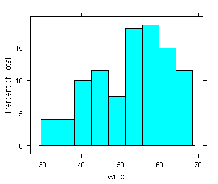
#histograms
histogram(~write, hsb2)
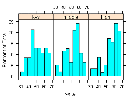
#conditional plot
histogram(~write | ses.f, hsb2)
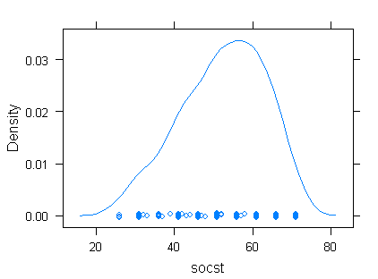
Density plots
densityplot(~socst, hsb2)
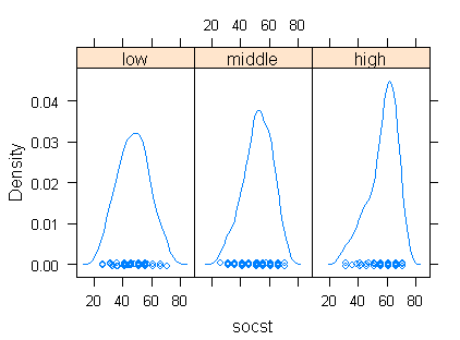
#conditional plot
densityplot(~socst | ses.f, hsb2)
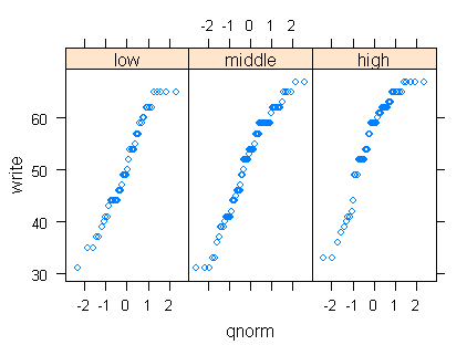
Quantile-quantile plots
qqmath(~write, hsb2)
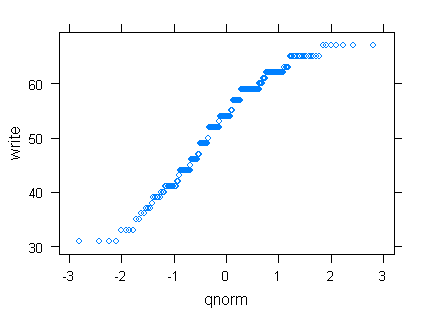
#conditional plot
qqmath(~write | ses.f, hsb2)
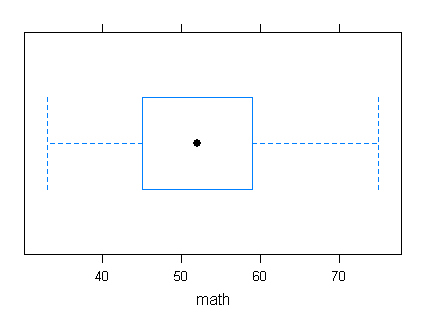
Box and whiskers plots
bwplot(~math, hsb2)
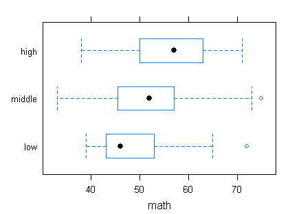
#conditional plot
bwplot(ses.f~math, hsb2)
2. Multivariate Plots
Scatter plots
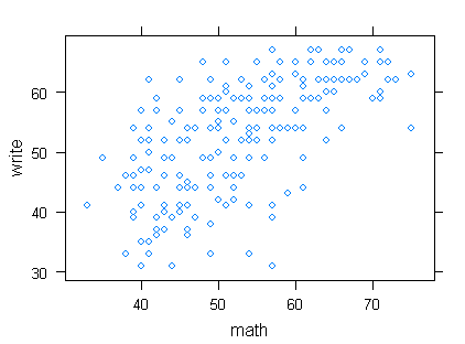
xyplot(write~math, hsb2)
#conditional plot
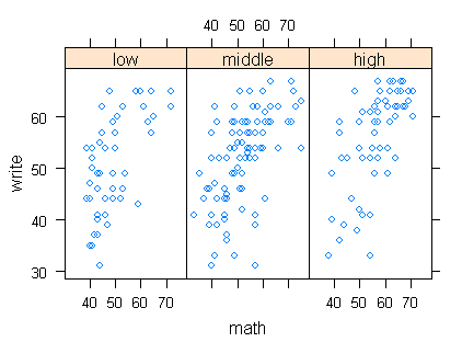
xyplot(write~math | ses.f, hsb2)
Scatter plot matrices
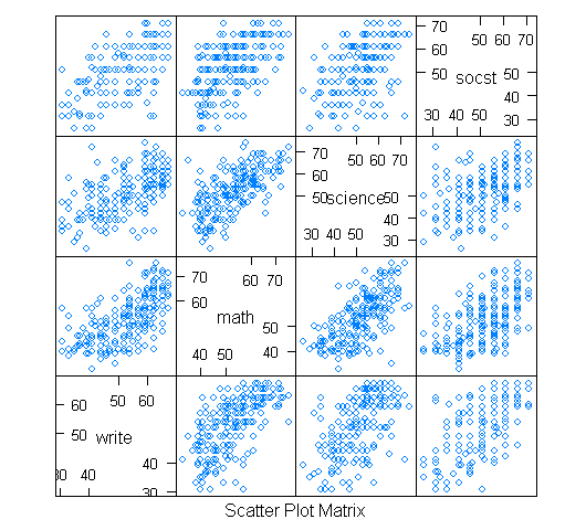
subset <- hsb2[ , 8:12]
splom(~subset[ , 1:4])
#conditional plot
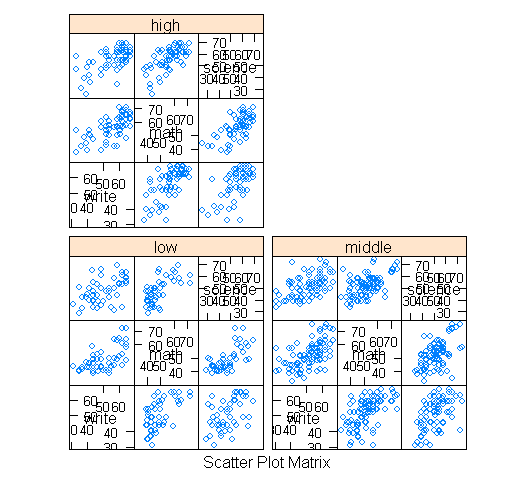
splom(~subset[, 1:3] | subset[, 5])
3. Examples of Plots Used in Statistical Analysis
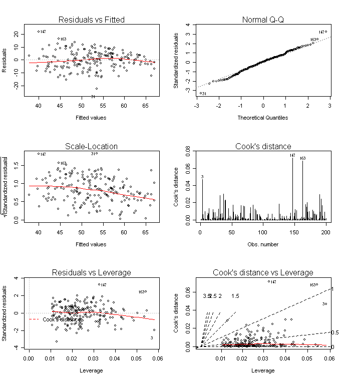
In regression analysis it can be very helpful to use diagnostic plots to assess the fit of the model. In
R there are a number of built in plots that can be accessed with minimal
effort or code.
reg <- lm(write~math+socst+ses.f, hsb2)
par(mfrow=c(3,2))
plot(reg, which=1:2)
plot(reg, which=3:4)
plot(reg, which=5:6)
detach(hsb2)