Factor variables
Version info: Code for this page was tested in R version 3.0.2 (2013-09-25)
On: 2013-11-27
With: knitr 1.5
1. Creating factor variables
Factor variables are categorical variables that can be either numeric or string variables. There are a number of advantages to converting categorical variables to factor variables. Perhaps the most important advantage is that they can be used in statistical modeling where they will be implemented correctly, i.e., they will then be assigned the correct number of degrees of freedom. Factor variables are also very useful in many different types of graphics. Furthermore, storing string variables as factor variables is a more efficient use of memory. To create a factor variable we use the factor function. The only required argument is a vector of values which can be either string or numeric. Optional arguments include the levels argument, which determines the categories of the factor variable, and the default is the sorted list of all the distinct values of the data vector. The labels argument is another optional argument which is a vector of values that will be the labels of the categories in the levels argument. The exclude argument is also optional; it defines which levels will be classified as NA in any output using the factor variable.
First we will generate a vector of numeric data called schtyp. It involves the random number generator so we will set the seed to equal 124 in order to make the results reproducible.
set.seed(124)
schtyp <- sample(0:1, 20, replace = TRUE)
schtyp
## [1] 0 0 1 0 0 0 1 0 1 0 1 1 1 1 0 0 1 1 1 0
is.factor(schtyp)
## [1] FALSE
is.numeric(schtyp)
## [1] TRUE
Now let’s create a factor variable called schtyp.f based on schtyp. The first label, private, will correspond to schtyp=0 and the second label, public, will correspond to schtyp=1 because the order of the labels will follow the numeric order of the data.
schtyp.f <- factor(schtyp, labels = c("private", "public"))
schtyp.f
##  [1] private private public  private private private public  private
##  [9] public  private public  public  public  public  private private
## [17] public  public  public  private
## Levels: private public
is.factor(schtyp.f)
## [1] TRUE
Let’s generate a string variable called ses (socio-economic status).
ses <- c("low", "middle", "low", "low", "low", "low", "middle", "low", "middle",
    "middle", "middle", "middle", "middle", "high", "high", "low", "middle",
    "middle", "low", "high")

is.factor(ses)
## [1] FALSE
is.character(ses)
## [1] TRUE
Creating a factor variable ses.f.bad.order based on ses.
ses.f.bad.order <- factor(ses)
is.factor(ses.f.bad.order)
## [1] TRUE
levels(ses.f.bad.order)
## [1] "high" "low" "middle"
The problem is that the levels are ordered according to the alphabetical order of the categories of ses. Thus, “high” is the lowest level of ses.f.bad.order, “middle” is the middle level and “low” is the highest level. In order to fix the ordering we need to use the levels argument to indicate the correct ordering of the categories. Let’s create a new factor variable called ses.f with the correct order of categories.
ses.f <- factor(ses, levels = c("low", "middle", "high"))
is.factor(ses.f)
## [1] TRUE
levels(ses.f)
## [1] "low" "middle" "high"
2. Creating ordered factor variables
We can create ordered factor variables by using the function ordered. This function has the same arguments as the factor function. Let’s create an ordered factor variable called ses.order based on the variable ses created in the above example.
ses.order <- ordered(ses, levels = c("low", "middle", "high"))
ses
##  [1] "low"    "middle" "low"    "low"    "low"    "low"    "middle"
##  [8] "low"    "middle" "middle" "middle" "middle" "middle" "high"
## [15] "high"   "low"    "middle" "middle" "low"    "high"
ses.order
##  [1] low    middle low    low    low    low    middle low    middle
## [10] middle middle middle middle high   high   low    middle middle
## [19] low    high
## Levels: low < middle < high
is.factor(ses.order)
## [1] TRUE
3. Adding and dropping levels in factor variables
Below we will add an element from a new level (“very.high”) to ses.f our existing factor variable, ses.f. The number in the square brackets ( [21] ) indicates the number of the element whose label we wish to change.
ses.f[21] <- "very.high"
## Warning: invalid factor level, NA generated
ses.f
##  [1] low    middle low    low    low    low    middle low    middle
## [10] middle middle middle middle high   high   low    middle middle
## [19] low    high
## Levels: low middle high
We can see that instead of changing from “high” to “very.high”, the label was changed from “high” to <NA>. To do this correctly, we need to first add the new level, “very.high”, to the factor variable ses.f which we do by using the factor function with the levels argument. Then we can finally add an element to the factor variable from the new level.
ses.f <- factor(ses.f, levels = c(levels(ses.f), "very.high"))
ses.f[21] <- "very.high"
ses.f
##  [1] low       middle    low       low       low       low
##  [7] middle    low       middle    middle    middle    middle
## [13] middle    high      high      low       middle    middle
## [19] low       high      very.high
## Levels: low middle high very.high
levels(ses.f)
## [1] "low" "middle" "high" "very.high"
Dropping a level of a factor variable is a little easier. The simplest way is to first remove all the elements within the level to be removed and then to redeclare the variable to be a factor variable. (The level is not automatically removed if there are no elements in it because we could just by chance have a sample which did not contain elements from a specific level.) Let’s illustrate this by removing the level of “very.high” from the ses.f variable.
ses.f.new <- ses.f[ses.f != "very.high"]
ses.f.new
##  [1] low    middle low    low    low    low    middle low    middle
## [10] middle middle middle middle high   high   low    middle middle
## [19] low    high
## Levels: low middle high very.high
ses.f.new <- factor(ses.f.new)
ses.f.new
##  [1] low    middle low    low    low    low    middle low    middle
## [10] middle middle middle middle high   high   low    middle middle
## [19] low    high
## Levels: low middle high
levels(ses.f.new)
## [1] "low" "middle" "high"
4. Examples of the usefulness of factor variables
To illustrate the usefulness of factor variables we are first going to create a data frame with all the variables we have used in the previous examples, plus an additional continuous variable called read which contains the reading scores. We also redefine ses.f to equal the ses.f.new variable which does not have any “very.high” elements.
ses.f <- ses.f.new
read <- c(34, 39, 63, 44, 47, 47, 57, 39, 48, 47, 34, 37, 47, 47, 39, 47,
    47, 50, 28, 60)

# combining all the variables in a data frame
combo <- data.frame(schtyp, schtyp.f, ses, ses.f, read)
Tables are much easier to interpret when using factor variables because they add useful labels to the table and they arrange the factors in a more understandable order.
table(ses, schtyp)
##         schtyp
## ses      0 1
##   high   2 1
##   low    6 2
##   middle 2 7
table(ses.f, schtyp.f)
##         schtyp.f
## ses.f    private public
##   low          6      2
##   middle       2      7
##   high         2      1
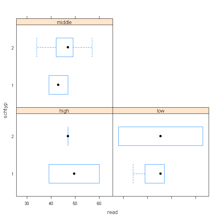
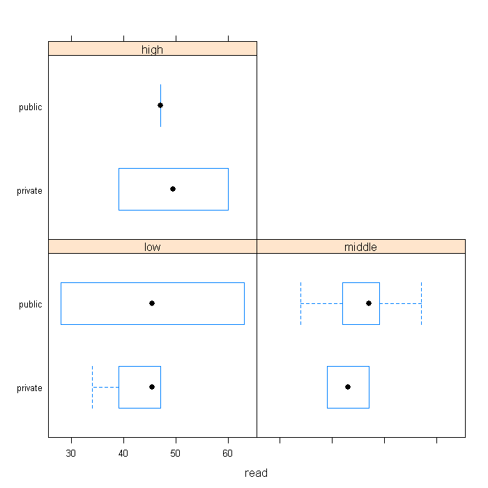
Graphics are another area that benefits from the use of factor variables. As in the tables the factor variable will indicate a better ordering of the graphs as well as add useful labels.
library(lattice)
bwplot(schtyp ~ read | ses, data = combo, layout = c(2, 2))

bwplot(schtyp.f ~ read | ses.f, data = combo, layout = c(2, 2))

