Version info: Code for this page was tested in R version 3.0.2 (2013-09-25)
On: 2013-11-19
With: lattice 0.20-24; foreign 0.8-57; knitr 1.5
1. Generating random samples from a normal distribution
Even though we would like to think of our samples as random, it is in fact almost impossible to generate random numbers on a computer. So, we will admit that we are really drawing a pseudo-random sample. In order to be able to reproduce the results on this page we will set the seed for our pseudo-random number generator to the value of 124 using the set.seed function. (For more information on the random number generator used in R please refer to the help pages for the Random.Seed function which has a very detailed explanation.)
set.seed(124)
It is often very useful to be able to generate a sample from a specific distribution. To generate a sample of size 100 from a standard normal distribution (with mean 0 and standard deviation 1) we use the rnorm function. We only have to supply the n (sample size) argument since mean 0 and standard deviation 1 are the default values for the mean and stdev arguments.
norm <- rnorm(100)
Now let’s look at the first 10 observations. We use square brackets to surround the first and last element number. In the output, the number of the first element listed on the line is given in the square brackets. For example, the [9] indicates that the first number given (0.19709386) is the ninth element.
norm[1:10]
##  [1] -1.3851  0.0383 -0.7630  0.2123  1.4255  0.7445  0.7002 -0.2294
##  [9]  0.1971  1.2072
mean(norm)
## [1] 0.00962
sd(norm)
## [1] 0.884
If we want to obtain a sample of values drawn from a normal distribution with a different value for the mean and standard deviation then we just have to use the mean and sd arguments. Let’s draw a sample of size 100 from a normal distribution with mean 2 and standard deviation 5.
set.seed(124)
norm <- rnorm(100, 2, 5)
norm[1:10]
## [1] -4.925 2.192 -1.815 3.062 9.128 5.722 5.501 0.853 2.985 8.036
mean(norm)
## [1] 2.05
sd(norm)
## [1] 4.42
2. Generating random samples from other distributions
Here is a list of the functions that will generate a random sample from other common distributions: runif, rpois, rmvnorm, rnbinom, rbinom, rbeta, rchisq, rexp, rgamma, rlogis, rstab, rt, rgeom, rhyper, rwilcox, rweibull. Each function has its own set of parameter arguments. For example, the rpois function is the random number generator for the Poisson distribution and it has only the parameter argument lambda. The rbinom function is the random number generator for the binomial distribution and it takes two arguments: size and prob. The size argument specifies the number of Bernoulli trials and the prob argument specifies the probability of a success for each trial.
# Generating a random sample from a Poisson distribution with lambda=3
set.seed(124)
pois <- rpois(100, lambda = 3)
pois[1:10]
## [1] 1 2 3 2 2 2 3 3 6 2
mean(pois)
## [1] 2.83
var(pois)
## [1] 2.34
# Generating a random sample from a Binomial distribution with size=20 and
# prob=.2
set.seed(124)
binom <- rbinom(100, 20, 0.2)
binom[1:10]
## [1] 2 3 4 3 3 3 4 4 7 3
mean(binom)
## [1] 3.85
sd(binom)
## [1] 1.6
3. Other probability and distribution functions
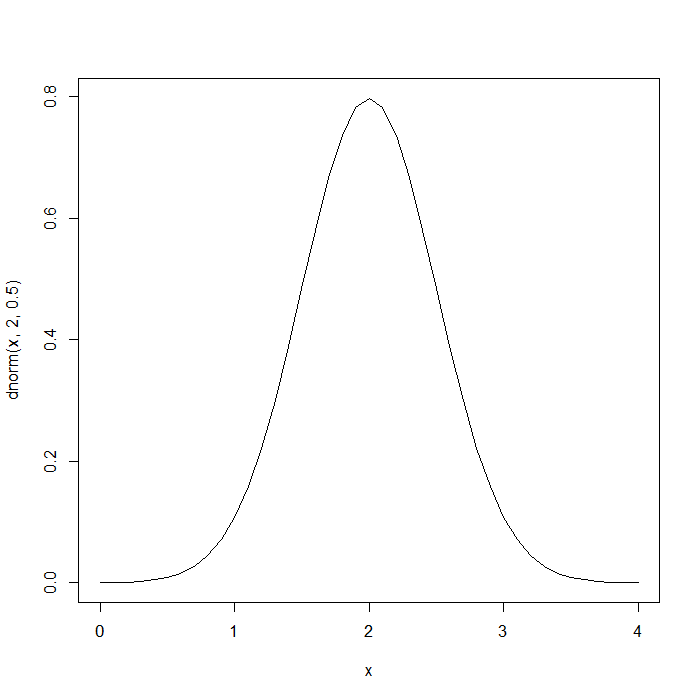
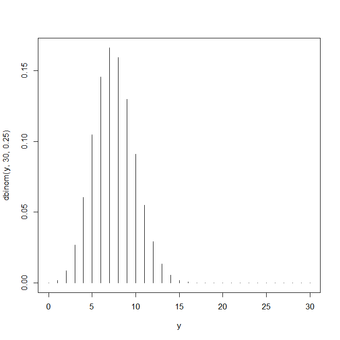
For each of the distributions there are four functions which will generate fundamental quantities of a distribution. Let’s consider the normal distribution as an example. We have already given examples of the rnorm function which will generate a random sample from a specific normal distribution. The dnorm function will generate the density (or point) probability for a specific value for a normal distribution. This function is very useful for creating a plot of a density function of a distribution. In the list of the random number generator functions all the functions started with an “r”, similarly the density functions for all the distributions all start with a “d”.
# point probability for a specific value of a standard normal dist
dnorm(-1.96)
## [1] 0.0584
# plotting the density function of a normal distribution: N(2, .25)
x <- seq(0, 4, 0.1)

plot(x, dnorm(x, 2, 0.5), type = "l")

# plotting the density function of a binomial distribution: Binom(30, .25)
y <- 0:30
plot(y, dbinom(y, 30, 0.25), type = "h")

It is also possible to calculate p-values using the cumulative distribution functions. For the normal distribution this function is the pnorm and for the other distributions these functions all start with a “p”.
# calculating the p-values for the quantiles of a standard normal
1 - pnorm(1.959964)
## [1] 0.025
1 - pnorm(1.644854)
## [1] 0.05
It is also possible to calculate the quantiles for a specific distribution. For the normal distribution this function is the qnorm and for the other distribution these functions all start with a “q”.
# calculating the quantiles for the standard normal
qnorm(0.05)
## [1] -1.64
qnorm(0.025)
## [1] -1.96
4. The sample function
The sample function is used to generate a random sample from a given population. It can be used to sample with or without replacement by using the replace argument (the default is F). The only obligatory argument is a vector of data which will constitute the population from which the sample will be drawn. The default is to create a sample equal in size to the population but by using the size argument any sample size can be specified. A vector of probabilities can also be supplied in the prob argument. This vector has to be equal in length to the size of the population and it will automatically be normalized if its elements do not sum up to one. The default is for every element in the population to have equal chance of being chosen.
# random sample of size 8 from sequence [5, 15]
set.seed(124)

sample(seq(5, 15), 8)
## [1] 5 9 14 8 6 11 7 10
# random permutation of sequence [1, 10]
set.seed(124)

sample(10)
## [1] 1 4 5 3 2 6 7 8 9 10
# random sample of size 10 from sequence [1, 5] with unequal probabilities
# of being chosen
set.seed(124)

sample(5, 10, prob = c(0.3, 0.4, 0.1, 0.1, 0.1), replace = T)
## [1] 2 1 1 2 2 2 1 1 4 2
