
Purpose
This seminar will introduce basic concepts of structural equation modeling using lavaan in the R statistical programming language. Its emphasis is on identifying various manifestations of SEM models and interpreting the output rather than a thorough mathematical treatment or a comprehensive list of syntax options in lavaan. Since SEM is a broad topic, only the most fundamental topics such as matrix notation, identification and model fit will be introduced in this seminar. Topics such as estimation, multiple groups, measurement invariance and latent growth modeling will not be covered in this seminar. The assumption is that all variables are continuous and normally distributed.
This seminar is the second in a three-part series on latent variable modeling. The first seminar of this seminar introduces CFA:
The third seminar introdues intermediate topics in CFA including latent growth modeling and measurement invariance:
For exploratory factor analysis (EFA), please refer to A Practical Introduction to Factor Analysis: Exploratory Factor Analysis.
In addition to the pre-requisites above, a rudimentary knowledge of linear regression is required to understand some of the material in this seminar.
Outline
Proceed through the seminar in order or click on the hyperlinks below to go to a particular section:
- Simple regression (Model 1A)
- Maximum likelihood vs. least squares
- Multiple regression (Model 2)
- Multivariate regression with default covariance (Model 3A)
- Multivariate regression removing default covariances (Model 3D)
- Fully saturated Multivariate Regression (Model 3E)
- Known values, parameters, and degrees of freedom
- Path analysis (Model 4A)
- Modification index
- Path analysis after modification (Model 4B)
- Model chi-square
- A note on sample size
- The baseline model
- CFI (Comparative Fit Index)
- TLI (Tucker Lewis Index)
- RMSEA
- Structural Regression Model
- Structural regression with one endogenous variable (Model 6A)
- Structural regression with two endogenous variables (Model 6B)
- (Optional) Structural regression with an observed endogenous variable (Model 6C)
- Conclusion
- References
Requirements
Before beginning the seminar, please make sure you have R and RStudio installed.
Please also make sure to have the following R package installed, and if not, run these commands in R (RStudio).
install.packages("lavaan", dependencies=TRUE)
Once you’ve installed the package, you can load lavaan via the following
library(lavaan)
Download the complete R code
You may download the complete R code here: sem.r
After clicking on the link, you can copy and paste the entire code into R or RStudio.
Introduction
Structural equation modeling is a linear model framework that models both simultaneous regression equations with latent variables. Models such as linear regression, multivariate regression, path analysis, confirmatory factor analysis, and structural regression can be thought of as special cases of SEM. The following relationships are possible in SEM:
- observed to observed variables ($\gamma$, e.g., regression)
- latent to observed variables ($\lambda$, e.g., confirmatory factor analysis)
- latent to latent variables ($\gamma,\beta$ e.g., structural regression)
SEM uniquely encompasses both measurement and structural models. The measurement model relates observed to latent variables and the structural model relates latent to latent variables. Various software programs currently handle SEM models including Mplus, EQS, SAS PROC CALIS, Stata’s sem and more recently, R’s lavaan. The benefit of lavaan is that it is open source, freely available, and is relatively easy to use.
This seminar will introduce the most common models that fall under the SEM framework including
- simple regression
- multiple regression
- multivariate regression
- path analysis
- confirmatory factor analysis
- structural regression
The purpose of the seminar will be to introduce within each model its
- matrix formulation
- path diagram
lavaansyntax- interpretation of parameters and output
By the end of this training, you should be able to understand enough of these concepts to correctly identify the model, recognize each parameter in the matrix formulation and interpret the output of each model in lavaan. Finally, for those of you who are interested, the technical underpinnings of all these models are based on classic LISREL (linear structural relations) notation in honor of Karl Joreskög (1969, 1973). Although critics of LISREL note its complexity and sharp learning curve for the causal user, all modern implementations of SEM are derivations of LISREL and serve either to expand its capabilities or whittle down its complexity. Thus understanding LISREL is foundational to understanding more modern SEM frameworks and programs.
Motivating example
Suppose you are a researcher studying the effects of student background on academic achievement. The lab recently finished collecting and uploading the dataset (worland5.csv) of $N=500$ students each with 9 observed variables: Motivation, Harmony, Stability, Negative Parental Psychology, SES, Verbal IQ, Reading, Arithmetic and Spelling. The principal investigator hypothesizes three latent constructs Adjustment, Risk, Achievement measured with its corresponding to the following codebook mapping:
Adjustment
motivMotivationharmHarmonystabiStability
Risk
ppsych(Negative) Parental PsychologysesSESverbalVerbal IQ
Achievement
readReadingarithArithmeticspellSpelling
Due to budget constraints, your lab uses the freely available R statistical programming language, and lavaan as the structural equation modeling (SEM) package of choice. You can download the file from the link here worland5.csv or load the file directly into R with the following command
dat <- read.csv("https://stats.idre.ucla.edu/wp-content/uploads/2021/02/worland5.csv")
The most essential component of a structural equation model is covariance or the statistical relationship between items. The true population covariance, denoted $\Sigma$, is called the variance-covariance matrix. Since we do not know $\Sigma$ we can estimate it with our sample, and call it $\hat{\Sigma}=S$, or the sample variance-covariance matrix. The function cov specifies that we want to obtain the covariance matrix $S$ from the data.
> cov(dat)
       motiv harm stabi ppsych ses verbal read arith spell
motiv    100   77    32    -25  25     59   53    60    59
harm      77  100    25    -25  26     58   42    44    45
stabi     32   25   100    -40  40     27   56    49    48
ppsych   -25  -25   -40    100 -42    -16  -39   -24   -31
ses       25   26    40    -42 100     18   43    37    33
verbal    59   58    27    -16  18    100   36    38    38
read      53   42    56    -39  43     36  100    73    87
arith     60   44    49    -24  37     38   73   100    72
spell     59   45    48    -31  33     38   87    72   100
Both $\Sigma$ and $S$ share similar properties. The diagonals constitute the variances of the item and the off-diagonals the covariances. Notice that the variance of all variables in our study happens to be 100 (down the diagonals). Looking at the relationships between variables (the off-diagonal elements), recall that a positive covariance means that as one item increases the other increases, a negative covariance means that as one item increases the other item decreases. The covariance of motiv and ppsych is -25 which means that as negative parental psychology increases student motivation decreases. Notice that the covariances in the upper right triangle are the same as those in the lower right triangle, meaning the covariance of Motivation and Harmony is the same as the covariance of Harmony and Motivation. This property is known as symmetry and will be important later on. The variance-covariance matrix $\Sigma$ should not be confused with $\Sigma{(\theta)}$ which is the model-implied covariance matrix. The purpose of SEM is to reproduce the variance-covariance matrix using parameters $\theta$ we hypothesize will account for either the measurement or structural relations between variables. If the model perfectly reproduces the variance-covariance matrix then $\Sigma=\Sigma{(\theta)}$.
True or False. Running the cov command in R allows us to obtain the population variance-covariance matrix $\Sigma$
Answer: False, since we are running our analysis on a sample we are obtaining $S$.
True or False. $S=\hat{\Sigma}$ means that it is an estimate of the population variance-covariance matrix.
Answer: True, the hat symbol indicates an estimate
True or False. $\Sigma{(\theta)}$ is the variance-covariance matrix reproduced from model parameters
Answer: True, $\theta$ denotes model parameters. The goal of SEM is to reproduce $\Sigma$ with $\Sigma{(\theta)}$.
Definitions
- observed variable: a variable that exists in the data, a.k.a item or manifest variable
- latent variable: a variable that is constructed and does not exist in the data
- exogenous variable: an independent variable either observed (x) or latent ($\xi$) that explains an endogenous variable
- endogenous variable: a dependent variable, either observed (y) or latent ($\eta$) that has a causal path leading to it
- measurement model: a model that links observed variables with latent variables
- indicator: an observed variable in a measurement model (can be exogenous or endogenous)
- factor: a latent variable defined by its indicators (can be exogenous or endogenous)
- loading: a path between an indicator and a factor
- structural model: a model that specifies causal relationships among exogenous variables to endogenous variables (can be observed or latent)
- regression path: a path between exogenous and endogenous variables (can be observed or latent)
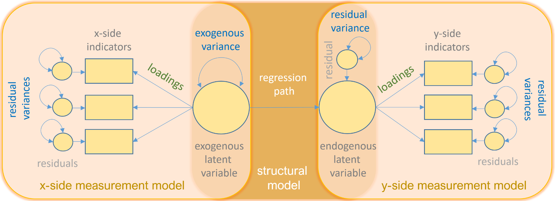
There is subtlety to the definition of an indicator. Although $x$ variables are typically seen as independent variables in a linear regression, the $x$ or $y$ label of an indicator in a measurement model depends on the factor it belongs to. An indicator is an $x$-side indicator if it depends on an exogenous factor and a $y$-side indicator if it depends on an endogenous factor.
True or False. If an observed $x$-variable is being predicted by an endogenous factor, then it is called an $x$-side indicator.
Answer: False. If an indicator is being predicted by an endogenous factor, it is a $y$-side indicator and should be relabeled $y$.
True or False. Because an $x$-variable is being predicted by a factor, it is a dependent variable and should be relabeled $y$.
Answer: False. Both $x$-side and $y$-side variables are dependent variables, but whether it is $x$-side or $y$-side depends on the endogenity of its factor.
The path diagram
To facilitate understanding of the matrix equations (which can be a bit intimidating), a path diagram will be presented with every matrix formulation as it is a symbolic one-to-one visualization. Before we present the actual path diagram, the table below defines the symbols we will be using. Circles represent latent variables, squares represent observed indicators, triangles represent intercepts or means, one-way arrows represent paths and two-way arrows represent either variances or covariances.
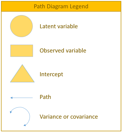
For example in the figure below, the diagram on the left depicts the regression of a factor on an item (contained in a measurement model) and the diagram on the right depicts the variance of the factor (a two-way arrow pointing to a the factor itself).

The following is a path diagram of all the types of variables and relationships you will see in this seminar.
Quick reference of lavaan syntax
Before running our first regression analysis, let us introduce some of the most frequently used syntax in lavaan
~predict, used for regression of observed outcome to observed predictors (e.g.,y ~ x)=~indicator, used for latent variable to observed indicator in factor analysis measurement models (e.g.,f =~ q + r + s)~~covariance (e.g.,x ~~ x)~1intercept or mean (e.g.,x ~ 1estimates the mean of variablex)1*fixes parameter or loading to one (e.g.,f =~ 1*q)NA*frees parameter or loading (useful to override default marker method, (e.g.,f =~ NA*q)a*labels the parameter ‘a’, used for model constraints (e.g.,f =~ a*q)
Regression and Path Analysis
Simple regression (Model 1A)
Simple regression models the relationship of an observed exogenous variable on a single observed endogenous variable. For a single subject, the simple linear regression equation is most commonly defined as:
$$y_1 = b_0 + b_1 x_1 + \epsilon_1$$
where $b_0$ is the intercept and $b_1$ is the coefficient and $x$ is an observed predictor and $\epsilon$ is the residual. Karl Joreskög, the originator of LISREL (linear structural relations), developed a special notation for the exact same model for a single observation:
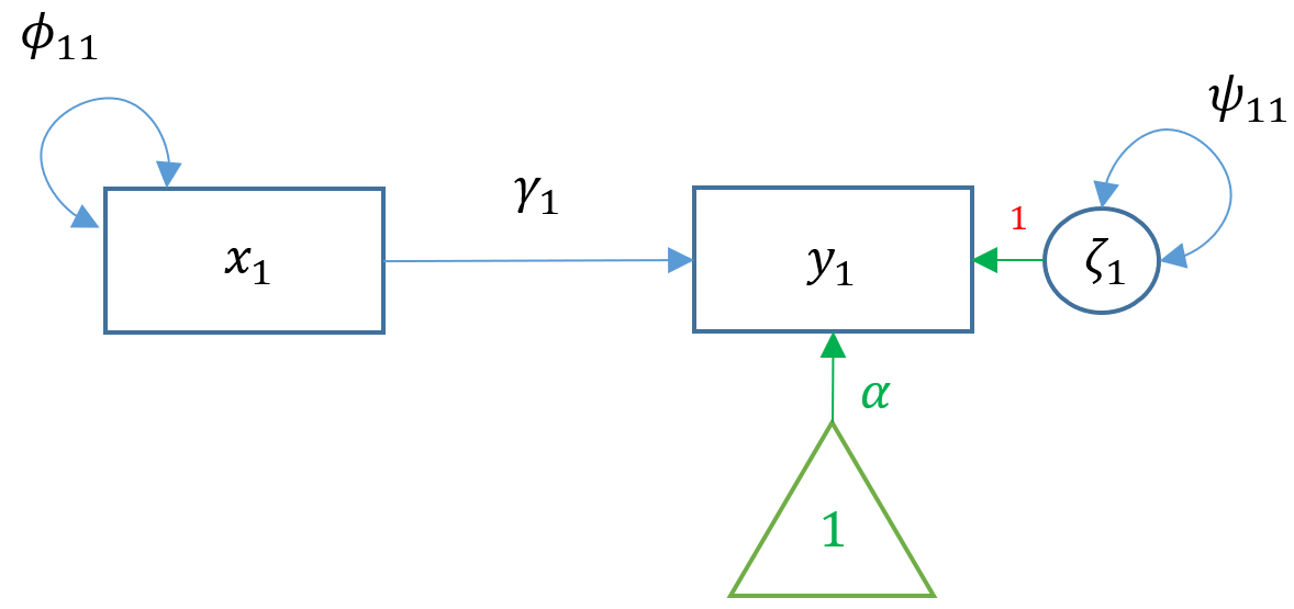
$$y_1 = \alpha + \gamma x_1 + \zeta_1$$
Definitions
- $x_1$ single exogenous variable
- $y_1$ single endogenous variable
- $b_0, \alpha_1$ intercept of $y_1$, “alpha”
- $b_1, \gamma_1$ regression coefficient, “gamma”
- $\epsilon_1, \zeta_1$ residual of $y_1$, “epsilon” and “zeta”
- $\phi$, variance or covariance of the exogenous variable, “phi”
- $\psi$ residual variance or covariance of the endogenous variable, “psi”
True or False. In Model 1A above, there is one endogenous outcome and one exogenous predictor.
Answer: True.
True or False. In Model 1A above, $y_1$ means that I have 1 observation (i.e., student) in my sample
Answer: False. $y_1$ indicates that there is one endogenous variable with $N$ samples.
To see the matrix visually, we can use a path diagram (Model 1A):
In R, the most basic way to run a linear regression is to use the lm() function which is available in base R.
#simple regression using lm()
m1a <- lm(read ~ motiv, data=dat)
(fit1a <-summary(m1a))
The output of lm() appears as below:
Coefficients:
              Estimate Std. Error t value Pr(>|t|)
(Intercept) -1.232e-07  3.796e-01    0.00        1
motiv        5.300e-01  3.800e-02   13.95   <2e-16 ***
---
Signif. codes:  0 ‘***’ 0.001 ‘**’ 0.01 ‘*’ 0.05 ‘.’ 0.1 ‘ ’ 1

Residual standard error: 8.488 on 498 degrees of freedom
The predicted mean of read is 0 for a student with motiv=0 and for a one unit increase in motivation, the reading score improves 0.530 points. Make special note of the residual standard error which is $8.488$. The square of that $8.488^2=72.04$ is the residual variance, which we will see later in lavaan(). We can run the equivalent code in lavaan. The syntax is very similar to lm() in that read ~ motiv specifies the predictor motiv on the outcome read. However, by default the intercept is not included in the output but is implied. If we want to add an intercept, we need to include read ~ 1 + motiv. Optionally, you can request the variance of motiv using motiv ~~ motiv. If this syntax is not provided, the parameter is still estimated but just implied.
#simple regression using lavaan
m1b <-   '
  # regressions
    read ~ 1 + motiv
  # variance (optional)
    motiv ~~ motiv
'
fit1b <- sem(m1b, data=dat)
summary(fit1b)
The output appears as below:
> summary(fit1b)
lavaan 0.6-7 ended normally after 14 iterations

  Estimator                                         ML
  Optimization method                           NLMINB
  Number of free parameters                          5

  Number of observations                           500

Model Test User Model:

  Test statistic                                 0.000
  Degrees of freedom                                 0

Parameter Estimates:

  Standard errors                             Standard
  Information                                 Expected
  Information saturated (h1) model          Structured

Regressions:
                   Estimate  Std.Err  z-value  P(>|z|)
  read ~
    motiv             0.530    0.038   13.975    0.000

Intercepts:
                   Estimate  Std.Err  z-value  P(>|z|)
   .read             -0.000    0.379   -0.000    1.000
    motiv             0.000    0.447    0.000    1.000

Variances:
                   Estimate  Std.Err  z-value  P(>|z|)
    motiv            99.800    6.312   15.811    0.000
   .read             71.766    4.539   15.811    0.000
The intercept of .read (-0.000) and the regression coefficient of read ~ motiv (0.530) matches the output of lm() with small rounding errors. Note that the . in front of the parameter denotes an endogenous variable under Intercepts and a residual variance if under Variances or Covariances. The intercept for motiv (0.000) does not have a . nor does its variance (99.800) signifying that it is an exogenous mean and variance. The exogenous mean and variance $\phi_{11}$ should closely match the univariate mean (0) and variance (100) as shown below:
> mean(dat$motiv)
[1] 2.4e-07
> var(dat$motiv)
[1] 100
Exercise
Match every parameter estimate to its corresponding path diagram shown above. Why is the intercept of motiv zero? What is the parameter that is not shown by default in lavaan?
Answer: : $y$=read, $x$=motiv, $\gamma_1=0.53$, $\alpha=0$, $\psi_{11}=71.766$. The intercept is zero because the researcher decided to center all variables at zero. The exogenous variance $\phi_{11}$ is not shown but is implicitly estimated, but we specified motiv ~~ motiv to explicitly model it.
Exercise
Try running the simple regression without the 1+. What do you notice about the number of free parameters and degrees of freedom?
Answer: : The number of free parameters decreases by 1 because we were estimating an additional intercept but this does not change the degrees of freedom because we are simply subtracting another term to the total parameters. Linear regression models are always saturated.
The important output to note is that the estimator is ML for Maximum Likelihood. Linear regression by default uses the least square estimator. As we will see below the coefficients will be the same but the residual variances will be slightly different. Additionally, there is default output for Variances, which is $71.766$.
Maximum likelihood vs. least squares
The estimates of the regression coefficients are equivalent between the two methods but the variance differs. For least squares, the estimate of the residual variance is:
$$ \hat{\sigma}^2_{LS} = \frac{\sum_{i=1}^{N} \hat{\zeta_i}^2}{N-k} $$ where $N$ is the sample size, and $k$ is the number of predictors + 1 (intercept)
For maximum likelihood the estimate of the residual variance is:
$$ \hat{\sigma}^2_{ML} = \frac{\sum_{i=1}^{N} \hat{\zeta_i}^2}{N} $$
To convert from the least squares residual variance to maximum likelihood:
$$ \hat{\sigma}^2_{ML} = \left(\frac{N-k}{n}\right) \hat{\sigma}^2_{LS} $$
Going back to the lm() output we see that
Residual standard error: 8.488 on 498 degrees of freedom
So the least square variance is $8.488^2=72.046$. To convert the variance to maximum likelihood, since $k=2$ we have $498/500(72.046)=71.76$.
> 498/500*(fit1a$sigma)**2
[1] 71.76618
This matches the lavaan output.
Variances:
                   Estimate  Std.Err  z-value  P(>|z|)
    motiv            99.800    6.312   15.811    0.000
   .read             71.766    4.539   15.811    0.000
True or False. The lm() function in R uses least squares estimation and lavaan uses maximum likelihood.
Answer: : True. These are the default estimation methods for each function; lavaan allows the user to change the estimation method such as generalized least squares (GLS) by specifying estimator=GLS. Refer to the lavaan documentation on Estimators for more information.
True or False. The fixed effects of an ordinary least squares regression is equivalent to maximum likelihood but the residual variance differs between the two.
Answer: : True.
Multiple regression (Model 2)
Simple regression is limited to just a single exogenous variable. In practice, a researcher may be interested in how a group of exogenous variable predict an outcome. Suppose we still have one endogenous outcome but two exogenous predictors; this is known as multiple regression (not to be confused with multivariate regression). Matrix form allows us to concisely represent the equation for all observations
$$y_1 = \alpha_1 + \mathbf{x \gamma} + \zeta_1$$
Definitions
- $y_1$ single endogenous variable
- $\alpha_1$ intercept for $y_1$
- $\mathbf{x}$ vector ($1 \times q$) of exogenous variables
- $\mathbf{\gamma}$ vector ($q \times 1$) of regression coefficients where $q$ is the total number of exogenous variables
- $\zeta_1$ residual of $y_1$, pronounced “zeta”.
- $\phi$, variance or covariance of the exogenous variable
- $\psi$ residual variance or covariance of the endogenous variable
Assumptions
- $E(\zeta)=0$ the mean of the residuals is zero
- $\zeta$ is uncorrelated with $\mathbf{x}$
Suppose we have two exogenous variables $x_1, x_2$ predicting a single endogenous variable $y_1$. The path diagram for this multiple regression (Model 2) is:

Specifying a multiple regression in lavaan is as easy as adding another predictor. Suppose the researcher is interested in how Negative Parental Psychology ppsych and Motivation motiv to predict student readings scores read.
m2 <- '
  # regressions
    read ~ 1 + ppsych + motiv
 # covariance
    ppsych ~~ motiv
'
fit2 <- sem(m2, data=dat)
summary(fit2)
The corresponding output is as follows. Compare the number of free parameters and degrees of freedom to the simple regression.
lavaan 0.6-7 ended normally after 34 iterations

  Estimator                                         ML
  Optimization method                           NLMINB
  Number of free parameters                          9

  Number of observations                           500

Model Test User Model:

  Test statistic                                 0.000
  Degrees of freedom                                 0

Parameter Estimates:

  Standard errors                             Standard
  Information                                 Expected
  Information saturated (h1) model          Structured

Regressions:
                   Estimate  Std.Err  z-value  P(>|z|)
  read ~
    ppsych           -0.275    0.037   -7.385    0.000
    motiv             0.461    0.037   12.404    0.000

Covariances:
                   Estimate  Std.Err  z-value  P(>|z|)
  ppsych ~~
    motiv           -24.950    4.601   -5.423    0.000

Intercepts:
                   Estimate  Std.Err  z-value  P(>|z|)
   .read              0.000    0.360    0.000    1.000
    ppsych           -0.000    0.447   -0.000    1.000
    motiv             0.000    0.447    0.000    1.000

Variances:
                   Estimate  Std.Err  z-value  P(>|z|)
   .read             64.708    4.092   15.811    0.000
    ppsych           99.800    6.312   15.811    0.000
    motiv            99.800    6.312   15.811    0.000
True or False. In Model 2, the vector $\alpha$ can be replaced with $\alpha_1$ as in the univariate regression model (Model 1A).
Answer: False. Unlike the univariate regression model (Model 1A) which has only one intercept, in multivariate regression, every outcome has its own intercept.
True or False. In Model 2 above, there are two $\gamma$’s because there are two exogenous variables. Given the same model, this would not change if we increased the sample size.
Answer: True, each endogenous variable gets its own regression model and can have as many exogenous variables as desired (theoretically). This is independent of the sample size.
Exercise
Re-run the analysis above without specifying ppsych ~~ motiv. Note the number of free parameters and degrees of freedom. Do the coefficients change? What does this imply?
Answer: : Degrees of freedom is still zero even though number of free parameters is 4. The extra parameters are the intercepts and variances of ppsych and motiv corresponding to $\kappa_{1}$ and $\kappa_{2}$ as well as $\phi_{11}$ and $\phi_{22}$. The covariance of ppsych and motiv $\phi_{12}$ which makes a total of five extra parameters. The total parameters is thus $4+5=9$.
Even though we increased our number of free parameters our degrees of freedom is still zero! We will explore why in the following section.
Multivariate regression (Models 3A-E)
Simple and multiple regression model one outcome ($y$) at a time. In multivariate or simultaneous linear regression, multiple outcomes $y_1,y_2,…,y_p$ are modeled simultaneously, where $q$ is the number of outcomes. The General Multivariate Linear Model is defined as
$$\mathbf{y} = \mathbf{\alpha} + \mathbf{\Gamma} \mathbf{x} + \mathbf{\zeta}$$
To see the matrix formulation more clearly, consider two (i.e., bivariate) endogenous variables ($y_1, y_2$) predicted by two exogenous predictors $x_1, x_2$.
$$
\begin{pmatrix}
y_{1} \\
y_{2}
\end{pmatrix}
=
\begin{pmatrix}
\alpha_1 \\
\alpha_2
\end{pmatrix}
+
\begin{pmatrix}
\gamma_{11} & \gamma_{12}\\
0 & \gamma_{22}
\end{pmatrix}
\begin{pmatrix}
x_1 \\
x_2
\end{pmatrix}
+
\begin{pmatrix}
\zeta_{1}\\
\zeta_{2}
\end{pmatrix}
$$
$\Gamma$ here is known as a structural parameter and defines the relationship of exogenous to endogenous variables.
Definitions
- $\mathbf{y} = (y_1, \cdots, y_p)’$ vector of $p$ endogenous variables (not the number of observations!)
- $\mathbf{x}= (x_1, \cdots, x_q)’$ vector of $q$ exogenous variables
- $\mathbf{\alpha}$ vector of $p$ intercepts
- $\Gamma$ matrix of regression coefficients ($p \times q$) linking endogenous to exogenous variables whose $i$-th row indicates the endogenous variable and $j$-th column indicates the exogenous variable
- $\mathbf{\zeta}= ( \zeta_1, \cdots, \zeta_p)’$ vector of $p$ residuals (for the number of endogenous variables not observations)
True or False. The size of the vector of residuals $\zeta$ in the model above is determined by the number of observations.
Answer: False. The size of $\zeta$ is determined by the number of endogenous variables $p$. This does not mean there is only one observation however. In reality there are $N \cdot p$ residuals but it’s not depicted in the model above.
True or False. $\gamma_{12}$ represents a regression coefficient of the second exogenous variable $x_2$ on the first outcome $y_1$.
Answer: True. The $i$-th row indicates the endogenous variable and $j$-th column indicates the exogenous variable.
True or False. $\Gamma$ is always a square matrix meaning the number of rows equals the number of columns
Answer: False, the rows of $\Gamma$ indicate the number of endogenous variables and the columns of $\Gamma$ indicate the number of exogenous variables. This matrix would only be square if the number of exogenous variables equals the number of endogenous variables.
Multivariate regression with default covariance (Model 3A)
Due to the added complexity of this and the following multivariate models, we will explicitly model intercepts in lavaan code but exclude them from the path diagrams. With that said, the path diagram for a multivariate regression model (Model 3A) is depicted as:
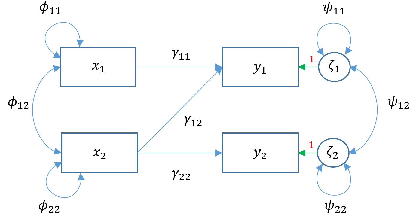 Here $x_1$
 ppsych and $x_2$ motiv predict $y_1$ read and only $x_2$ motiv predicts $y_2$ arith. The parameters $\phi_{11}, \phi_{22}$ represent the variance of the two exogenous variables respectively and $\phi_{12}$ is the covariance. Note that these parameters are modeled implicitly and not depicted in lavaan output. The parameters $\zeta_1, \zeta_2$ refer to the residuals of read and arith. Finally $\psi_{11},\psi_{22}$ represent the residual variances of read and arith and $\psi_{12}$ is its covariance. You can identify residual terms lavaan by noting a . before the term in the output.
True or False. The $y_1$ in the simple and multiple regression index one endogenous variable and in the multivariate outcome $y_1, y_2$ indexes two endogenous variables, not two samples.
Answer: True. If we had to index the number of observations in the multivariate regression, we would need two indexes for $y$, namely $y_{ij}$ where $i$ is the observation and $j$ the endogenous variable. For simplicity, we remove the index $i$ for the observations and simply focus on $j$.
True or False. Looking at Model 3A, $\psi_{11},\psi_{22}$ are the variances of $\zeta_1, \zeta_2$
Answer: True, they are the residual variances.
m3a <-
# regressions
read ~ 1 + ppsych + motiv
arith ~ 1 + motiv
'
fit3a <- sem(m3a, data=dat)
summary(fit3a)
The output is as follows:
lavaan 0.6-7 ended normally after 27 iterations

  Estimator                                         ML
  Optimization method                           NLMINB
  Number of free parameters                          8

  Number of observations                           500

Model Test User Model:

  Test statistic                                 6.796
  Degrees of freedom                                 1
  P-value (Chi-square)                           0.009

Parameter Estimates:

  Standard errors                             Standard
  Information                                 Expected
  Information saturated (h1) model          Structured

Regressions:
                   Estimate  Std.Err  z-value  P(>|z|)
  read ~
    ppsych           -0.216    0.030   -7.289    0.000
    motiv             0.476    0.037   12.918    0.000
  arith ~
    motiv             0.600    0.036   16.771    0.000

Covariances:
                   Estimate  Std.Err  z-value  P(>|z|)
 .read ~~
   .arith            39.179    3.373   11.615    0.000

Intercepts:
                   Estimate  Std.Err  z-value  P(>|z|)
   .read             -0.000    0.361   -0.000    1.000
   .arith            -0.000    0.357   -0.000    1.000

Variances:
                   Estimate  Std.Err  z-value  P(>|z|)
   .read             65.032    4.113   15.811    0.000
   .arith            63.872    4.040   15.811    0.000
As expected, the intercepts of read and arith are zero and its residual variances are 65.032 and 63.872. For multivariate regressions, the covariance of the residuals is given by default in lavaan and here estimated to be 39.179 (positive association between the variance of read and arith not accounted for by the exogenous variables. The relationship of read on ppsych is -0.216. For every one unit increase in Negative Parental Psychology, student Reading scores drop by 0.216 points controlling for the effects of student Motivation. The relationship of read on motivis 0.476 meaning as student Motivation increases by one unit, Reading scores increase by 0.476 points controlling for the effects of Negative Parental Psychology. Finally arith on motiv is 0.6; an increase of one point in student Motivation results in a 0.6 increase in Arithmetic scores.
Is multivariate regression the same as running two separate linear regressions? Let’s run lm() to find out. First let’s run model of read on ppsych and motiv.
m3b <- lm(read ~ ppsych + motiv, data=dat)
(fit3b <- summary(m3b))
The output is as follows:
Coefficients:
              Estimate Std. Error t value Pr(>|t|)
(Intercept) -1.336e-07  3.608e-01   0.000        1
ppsych      -2.747e-01  3.730e-02  -7.363 7.51e-13 ***
motiv        4.613e-01  3.730e-02  12.367  < 2e-16 ***
---
Signif. codes:
0 ‘***’ 0.001 ‘**’ 0.01 ‘*’ 0.05 ‘.’ 0.1 ‘ ’ 1

Residual standard error: 8.068 on 497 degrees of freedom
Multiple R-squared:  0.3516,	Adjusted R-squared:  0.349
F-statistic: 134.8 on 2 and 497 DF,  p-value: < 2.2e-16=
Now let’s run the model of arith on motiv in lm()
m3c <- lm(arith ~ motiv, data=dat)
(fit3c <- summary(m3c))
The output is as follows:
Coefficients:
              Estimate Std. Error t value Pr(>|t|)
(Intercept) -5.400e-08  3.581e-01    0.00        1
motiv        6.000e-01  3.585e-02   16.74   <2e-16 ***
---
Signif. codes:
0 ‘***’ 0.001 ‘**’ 0.01 ‘*’ 0.05 ‘.’ 0.1 ‘ ’ 1

Residual standard error: 8.008 on 498 degrees of freedom
Multiple R-squared:   0.36,	Adjusted R-squared:  0.3587
F-statistic: 280.1 on 1 and 498 DF,  p-value: < 2.2e-16
We see that the coefficients read ~~ ppsych is -0.216 in lavaan but -0.2747. Could this be rounding error? Furthermore, looking at the residual standard errors we see that the residual variance of arith is $8.008^2=64.12$ which is different from lavaan‘s estimate of $63.872$. Knowing what you know from the previous section, what could be the cause of this difference? We explore these questions in the following section.
Multivariate regression removing default covariances (Model 3D)
There are two facets to the question above. We already know previously that lm() uses the least squares estimator but lavaan uses maximum likelihood, hence the difference in residual variance estimates. However, regardless of which of the two estimators used, the regression coefficients should be unbiased so there must be something else accounting for the difference in coefficients. The answer lies in the implicit fact that lavaan by default will covary residual variances of endogenous variables .read ~~ .arith. Removing the default residual covariances, we see in the path diagram (Model 3D)
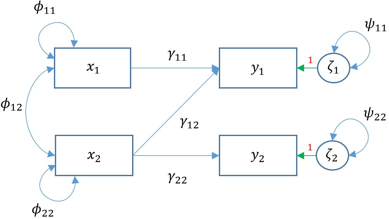
Removing the covariance of read and arith is the same as fixing its covariance to zero through the following syntax read ~~ 0*arith.
m3d <- '
  # regressions
    read ~ 1 + ppsych + motiv
    arith ~ 1 + motiv
  # covariance
    read ~~ 0*arith
'
fit3d <- sem(m3d, data=dat)
summary(fit3d)
The output is as follows:
lavaan 0.6-7 ended normally after 11 iterations

  Estimator                                         ML
  Optimization method                           NLMINB
  Number of free parameters                          7

  Number of observations                           500

Model Test User Model:

  Test statistic                               234.960
  Degrees of freedom                                 2
  P-value (Chi-square)                           0.000

Parameter Estimates:

  Standard errors                             Standard
  Information                                 Expected
  Information saturated (h1) model          Structured

Regressions:
                   Estimate  Std.Err  z-value  P(>|z|)
  read ~
    ppsych           -0.275    0.037   -7.385    0.000
    motiv             0.461    0.037   12.404    0.000
  arith ~
    motiv             0.600    0.036   16.771    0.000

Covariances:
                   Estimate  Std.Err  z-value  P(>|z|)
 .read ~~
   .arith             0.000

Intercepts:
                   Estimate  Std.Err  z-value  P(>|z|)
   .read             -0.000    0.360   -0.000    1.000
   .arith             0.000    0.357    0.000    1.000

Variances:
                   Estimate  Std.Err  z-value  P(>|z|)
   .read             64.708    4.092   15.811    0.000
   .arith            63.872    4.040   15.811    0.000
Notice now the coefficient of read on ppsych is -0.275 and read on motiv is 0.461. Compare now to the m3b
Coefficients:
              Estimate Std. Error t value Pr(>|t|)
(Intercept) -1.336e-07  3.608e-01   0.000        1
ppsych      -2.747e-01  3.730e-02  -7.363 7.51e-13 ***
motiv        4.613e-01  3.730e-02  12.367  < 2e-16 ***
Exercise
Compare the arith ~ motiv coefficient from m3c. Why do you think the coefficients are the same between lm() and lavaan ?
Answer: The residual variance is the variance that is not explained by all exogenous predictors in the model. The coefficients change between covariance on and off models if the additional exogenous variable is correlated with other endogenous variables. If the covariance is turned on then the residual variance will account for the effect of ppsych on arith that was not modeled. Any coefficients that are not modeled in the other regressions will appear in the residual covariances, hence the difference in the coefficients when covariances are turned off. Notice that motiv appears in bothread ~ motiv and arith ~ ppsych + motiv which means that turning the covariance on or off will result in the same coefficients.
Exercise
Re-run m3a and m3d with ppsych and motiv predicting both read and arith with covariances on and off. What do you notice about the coefficients?
Answer: Add the following syntax
read ~ 1 + ppsych + motiv
arith ~ 1 + ppsych + motiv
The coefficients for both models are the same
Regressions:
                   Estimate  Std.Err  z-value  P(>|z|)
  read ~
    ppsych           -0.275    0.037   -7.385    0.000
    motiv             0.461    0.037   12.404    0.000
  arith ~
    ppsych           -0.096    0.037   -2.616    0.009
    motiv             0.576    0.037   15.695    0.000
True or False. In lavaan, multivariate regression is equivalent to running to separate regressions.
Answer: : False. By default, lavaan correlates the residual variance of the endogenous variables. To make it equivalent, constrain this covariance to zero.
True or False. The reason the residual variances differ between Model 3D versus Models 3B,C is due to maximum likelihood vs. least squares estimation
Answer: True.
True or False. The variance term .arith in Model 3D is the variance of arithmetic itself. Compare this value to the variance calculated from Model 3C.
Answer: False. It is the residual variance. Note that even though we turned off the covariance, the estimate 63.872 differs from Model 3C’s estimate of the variance, which is the square of the residual standard error: 8.008^2 = 64.128.
Known values, parameters, and degrees of freedom
Both simple regression and multiple regression are saturated models which means that all parameters are fully estimated and there are no degrees of freedom. This is not necessarily true for multivariate regression models as Models 3A and 3D had degrees of freedom of 1 and 2 respectively. Let’s understand how the degrees of freedom is calculated. To begin, first count the number of known values in your observed population variance-covariance matrix $\Sigma$, given by the formula $p(p+1)/2$ where $p$ is the number of items in your survey. To see why this is true refer to the optional section Degrees of freedom with means from Confirmatory Factor Analysis (CFA) in R with lavaan for the more technically accurate explanation. Looking at the variables in the multivariate regression, we would like to obtain the variance-covariance matrix for Reading, Arithmetic, Parental Psychology and Motivation. To obtain the sample covariance matrix $S=\hat{\Sigma}$, which is an estimate of the population covariance matrix $\Sigma$, use the command cov and reference the column index of the dataset by name dat[,c("read","arith","ppsych","motiv")].
> cov(dat[,c("read","arith","ppsych","motiv")])
       read arith ppsych motiv
read    100    73    -39    53
arith    73   100    -24    60
ppsych  -39   -24    100   -25
motiv    53    60    -25   100
The off-diagonal cells in $S$ correspond to bivariate sample covariances between two pairs of items; and the diagonal cells in $S$ correspond to the sample variance of each item (hence the term “variance-covariance matrix“). Reading is positively related to Arithmetic, but Reading has a negative relationship with Parental Psychology. Just as in the larger covariance matrix we calculated before, the lower triangular elements in the covariance matrix are duplicated with the upper triangular elements. For example, the covariance of Reading with Arithmetic is 73, which is the same as the covariance of Arithmetic with Reading (recall the property of symmetry). Because the covariances are duplicated, the number of free parameters in SEM is determined by the number of unique variances and covariances. With 4 items, the number of known values is $p(p+1)/2 =4(5)/2=10$. The known values serve as the upper limit of the number of parameters you can possibly estimate in your model. The parameters coming from the model are called model parameters. Recall the multivariate model:
$$\mathbf{y = \alpha + \Gamma x + \zeta}$$
Since we care about the covariance of $y$, then by the assumption that $\alpha, x, \zeta$ are independent. Recall that covariance of a constant vector is zero since $Cov(\alpha)=E[(\alpha-E(\alpha))(\alpha-E(\alpha)]=E[0]=0$:
$$\Sigma(\theta)=Cov(\mathbf{y}) = Cov(\mathbf{\alpha} + \mathbf{\Gamma x} + \mathbf{\zeta}) = Cov(\mathbf{\alpha}) + Cov(\mathbf{\Gamma x}) + Cov(\mathbf{\zeta}) = \mathbf{\Gamma} Cov(\mathbf{x}) \mathbf{\Gamma}’ + \mathbf{\Psi} = \mathbf{\Gamma} \mathbf{\Phi} \mathbf{\Gamma}’ + \mathbf{\Psi}$$
This is a $2 \times 2$ matrix which serves as the upper left block of $\Sigma(\theta)$. Note that that full matrix of $\Sigma(\theta)$ here is $4 \times 4$. Since there are exactly two exogenous variables and two endogenous variables, each block is a $2 \times 2$ matrix.
$$
\Sigma(\theta) =
\begin{pmatrix}
\mathbf{\Gamma \Phi \Gamma’ + \Psi} & \mathbf{\Gamma \Phi}\\
\mathbf{\Phi \Gamma}’ & \mathbf{\Phi}
\end{pmatrix}
$$
However, since model parameters can be completely determined by elements of $y$, we do not consider parameters of $\Phi$ or $\Phi \Gamma’$. Spelling out the covariance matrix of $y$,
$$
\mathbf{\Gamma \Phi \Gamma’ + \Psi}
=
\begin{pmatrix}
\gamma_{11} & \gamma_{12} \\
\gamma_{21} & \gamma_{22}
\end{pmatrix}
\begin{pmatrix}
\phi_{11} & \phi_{12}\\
& \phi_{22}
\end{pmatrix}
\begin{pmatrix}
\gamma_{11} & \gamma_{21} \\
\gamma_{12} & \gamma_{22}
\end{pmatrix}
+
\begin{pmatrix}
\psi_{11} & \psi_{12}\\
& \psi_{22}
\end{pmatrix}
$$
Notice that the $\alpha$ does not appear in covariance model. First consider the dimensions of each parameter in Model 3A and 3D. Since there are two endogenous variables and exogenous variables $\Gamma$ is $2\times 2$ for a total of 4 parameters. For two exogenous variables, the dimension of $\Phi$ is $2 \times 2$ but by symmetry, $\phi_{12}=\phi_{21}$ which means we have 3 $\phi$’s. For two endogenous variables the dimension of $\Psi$ is also $2 \times 2$ but since $\psi_{12}=\psi_{21}$ there are a total of 3 $\psi$’s.
Then the total number of (unique) parameters here is $4 + 3 + 3 = 10$ parameters. It’s not a coincidence then that the number of model parameters matches the number of known values. If we estimate every possible parameter then this is by definition a saturated model (see Model 3E below).
True or False. $\Gamma$ is always a symmetric matrix.
Answer: False $\gamma_{12} \ne \gamma_{21}$. The first is the regression of $y_1$ on $x_1$ and the second is the regression of $y_2$ on $x_2$.
Example using Model 3A
For edification purposes, we will modify the syntax of Model 3A slightly (without going too deeply in technical details, this syntax models implied parameters explicitly and removes intercept parameters). You should now be able to match every term in this output to the path diagram.
m3aa <- '
 # regressions
   read ~ ppsych + motiv
   arith ~ motiv
 # variance and covariance
   ppsych ~~ ppsych
   motiv ~~ motiv
   ppsych ~~ motiv
'
fit3aa <- sem(m3aa, data=dat)
summary(fit3aa)
The output is as follows
lavaan 0.6-7 ended normally after 43 iterations

  Estimator                                         ML
  Optimization method                           NLMINB
  Number of free parameters                          9

  Number of observations                           500

Model Test User Model:

  Test statistic                                 6.796
  Degrees of freedom                                 1
  P-value (Chi-square)                           0.009

Parameter Estimates:

  Standard errors                             Standard
  Information                                 Expected
  Information saturated (h1) model          Structured

Regressions:
                   Estimate  Std.Err  z-value  P(>|z|)
  read ~
    ppsych           -0.216    0.030   -7.289    0.000
    motiv             0.476    0.037   12.918    0.000
  arith ~
    motiv             0.600    0.036   16.771    0.000

Covariances:
                   Estimate  Std.Err  z-value  P(>|z|)
  ppsych ~~
    motiv           -24.950    4.601   -5.423    0.000
 .read ~~
   .arith            39.179    3.373   11.615    0.000

Variances:
                   Estimate  Std.Err  z-value  P(>|z|)
    ppsych           99.800    6.312   15.811    0.000
    motiv            99.800    6.312   15.811    0.000
   .read             65.032    4.113   15.811    0.000
   .arith            63.872    4.040   15.811    0.000
Exercise
Use the output generated above to calculate the number of free parameters.
Answer: The number of unique model parameters is 10 and the number of fixed parameters is 1, namely we fixed $\gamma_{21}=0$
Fixed versus free parameters
However we know from the output of Model 3A that the number of free parameters is 9 rather than 10. This is due to the fact that we have allowed for fixed parameters which are parameters that are not estimated and pre-determined to have a specific value. Which parameter have we fixed (see Exercise above)?
The number of free parameters is defined as
$$\mbox{number of free parameters} = \mbox{number of (unique) model parameters } – \mbox{number of fixed parameters}.$$
The goal is to maximize the degrees of freedom (df) which is defined as
$$\mbox{df} = \mbox{number of known values } – \mbox{ number of free parameters}$$
How many degrees of freedom do we have now?
Answer: $10 – 9 = 1$
Models that are just-identified or saturated have df = 0, which means that the number of free parameters equals the number of known values in $\Sigma$. An under-identified model means that the number known values is less than the number of free parameters and an over-identified model means that the number of known values is greater than the number of free parameters. To summarize
- known < free implies degrees of freedom < 0 (under-identified, bad)
- known = free implies degrees of freedom = 0 (just identified or saturated, neither bad nor good)
- known > free implies degrees of freedom > 0 (over-identified, good)
True or False. Over-identified models are good because you have extra degrees of freedom to work with
Answer: True. Over-identified models are the reason we can assess model fit (to be discussed later).
True or False. Linear regression and multiple regression models are saturated models.
Answer: True. Calculate the degrees of freedom and you will see it is zero.
Quiz
Using what you now know, explain why the degrees of freedom in simple regression is zero (exclude the intercept).
Answer: There three model parameters without the intercept, $\gamma_1, \phi_{11}$ and $\psi_{11}$ and no fixed values. So the number of free parameters is $3-0=3$. Since there are $2(3)/2=3$ known values, the degrees of freedom is $3-3=0$.
Challenge
Why are there 5 free parameters in the output of m1b?
Answer: We included the intercept term of the endogenous variable, so the free parameters are $\alpha_1, \gamma_1, \phi_{11}$ and $\psi_{11}$. Although we did not discuss this, lavaan implicitly models the intercept of the exogenous variable $\kappa_1$ which makes a total of five free parameters.
Fully saturated Multivariate Regression (Model 3E)
Now that we know how to distinguish between over-identified and just-identified models, we understand that adding a single path of $\gamma_{21}$ turns Model 3A into a just-identified or fully saturated model which we call Model 3E.
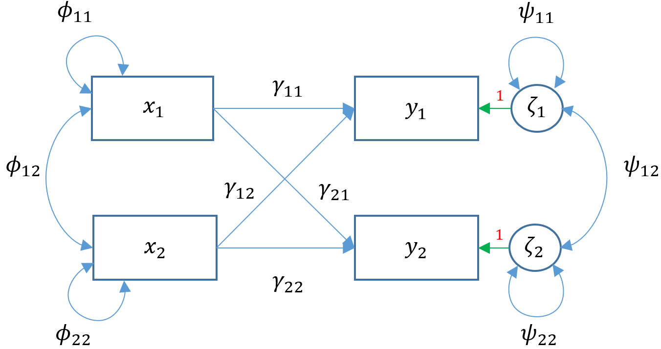
In lavaan, this is easy as adding the additional path of arith on ppsych but remembering that lavaan also by default models the covariance of $\psi_{12}$ which is the residual covariance between read and arith.
m3e <- '
  # regressions
    read ~ 1 + ppsych + motiv
    arith ~ 1 + ppsych + motiv
'
fit3e <- sem(m3e, data=dat)
summary(fit3e)
The output is as follows:
lavaan 0.6-7 ended normally after 29 iterations

  Estimator                                         ML
  Optimization method                           NLMINB
  Number of free parameters                          9

  Number of observations                           500

Model Test User Model:

  Test statistic                                 0.000
  Degrees of freedom                                 0

Parameter Estimates:

  Standard errors                             Standard
  Information                                 Expected
  Information saturated (h1) model          Structured

Regressions:
                   Estimate  Std.Err  z-value  P(>|z|)
  read ~
    ppsych           -0.275    0.037   -7.385    0.000
    motiv             0.461    0.037   12.404    0.000
  arith ~
    ppsych           -0.096    0.037   -2.616    0.009
    motiv             0.576    0.037   15.695    0.000

Covariances:
                   Estimate  Std.Err  z-value  P(>|z|)
 .read ~~
   .arith            38.651    3.338   11.579    0.000

Intercepts:
                   Estimate  Std.Err  z-value  P(>|z|)
   .read             -0.000    0.360   -0.000    1.000
   .arith            -0.000    0.355   -0.000    1.000

Variances:
                   Estimate  Std.Err  z-value  P(>|z|)
   .read             64.708    4.092   15.811    0.000
   .arith            63.010    3.985   15.811    0.000
We see that Negative Parental Psychology has a negative relationship with Arithmetic: for every one unit increase in the exogenous variable ppsych, the endogenous variable read decreases by 0.275.
Up to this point, we have explored multiple regression where one endogenous variable is predicted by two or more exogenous variables, multivariate regression where multiple exogenous variables can predict multiple endogenous variables. Finally, in the section to follow, we will see how path analysis allows endogenous variables to predict each other.
Path analysis (Model 4A)
Multivariate regression is a special case of path analysis where only exogenous variables predict endogenous variables. Path analysis is a more general model where all variables are still manifest but endogenous variables are allowed to explain other endogenous variables. Since $\Gamma$ specifies relations between an endogenous ($y$) and exogenous ($x$) variable, we need to create a new matrix $B$ that specifies the relationship between two endogenous ($y$) variables.
$$\mathbf{y = \alpha + \Gamma x + By + \zeta}$$
The matrix $B$ is a $p \times p$ matrix that is not necessarily symmetric. The rows of this matrix specify which $y$ variable is being predicted and the columns specify which $y$’s are predicting. For example, $\beta_{21}$ is in the second row meaning $y_2$ is being predicted and first column meaning $y_1$ is predicting.
True or False. $\beta_{21}$ is the same as $\beta_{12}$
Answer: False. In $\beta_{21}$ the endogenous variable $y_2$ is being predicted whereas $\beta_{12}$ means $y_1$ is being predicted.
Let’s extend our previous multivariate regression Model 3A so that we believe read which is an endogenous variable also predicts arith . Then the path diagram for Model 4A is shown below. What is the only path that is different between Model 3A and 4A?
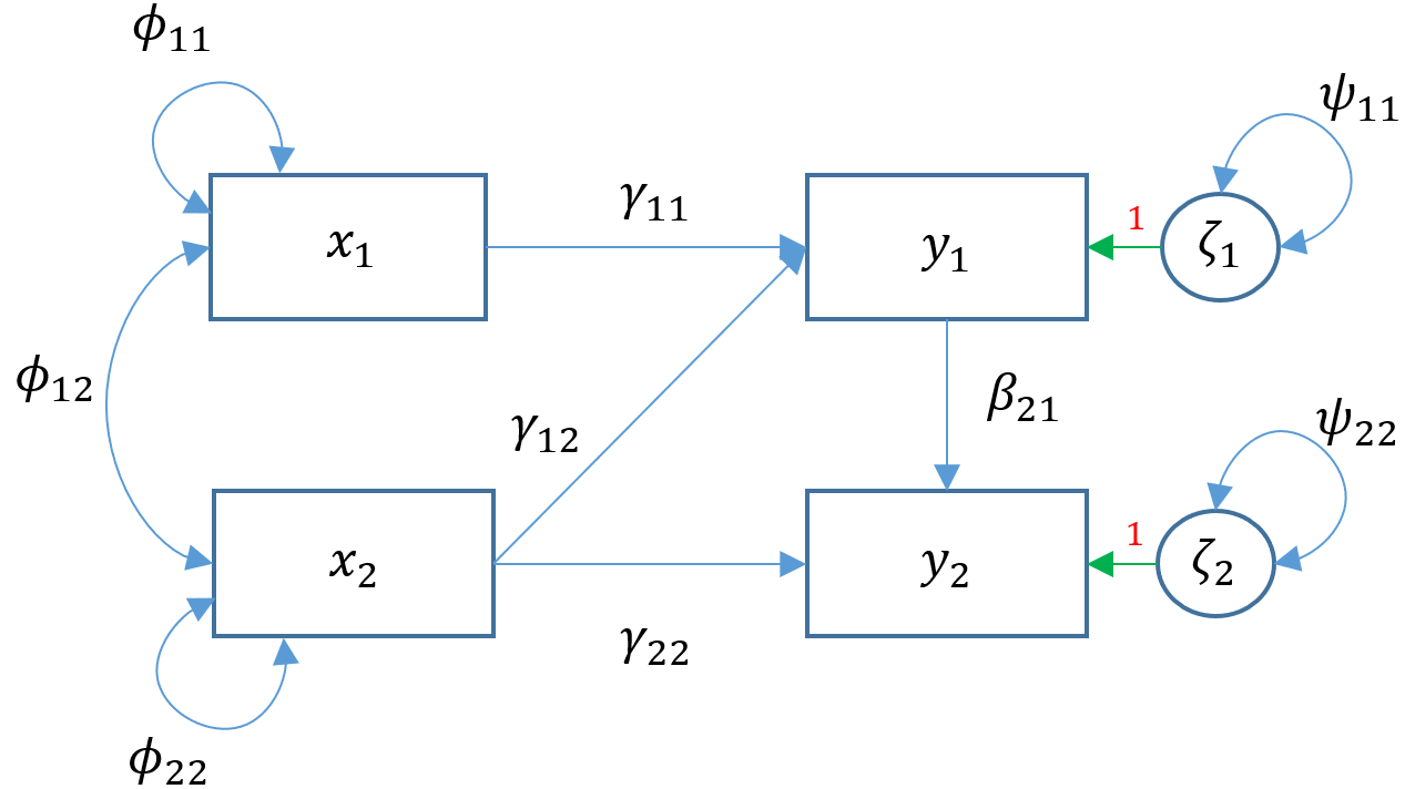
To see the matrix formulation for Model 4A, we have:
$$
\begin{pmatrix}
y_{1} \\
y_{2}
\end{pmatrix}
=
\begin{pmatrix}
\alpha_1 \\
\alpha_2
\end{pmatrix}
+
\begin{pmatrix}
\gamma_{11} & \gamma_{12}\\
0 & \gamma_{22}
\end{pmatrix}
\begin{pmatrix}
x_1 \\
x_2
\end{pmatrix}
+
\begin{pmatrix}
0 & 0\\
\beta_{21} & 0
\end{pmatrix}
\begin{pmatrix}
y_1 \\
y_2
\end{pmatrix}
+
\begin{pmatrix}
\zeta_{1}\\
\zeta_{2}
\end{pmatrix}
$$
Definitions
- $\mathbf{y} = (y_1, \cdots, y_p)’$ vector of $p$ endogenous variables
- $\mathbf{x} =(x_1, \cdots, x_q)’$ vector of $q$ exogenous variables
- $\mathbf{\alpha}$ vector of $p$ intercepts
- $\mathbf{\Gamma}$ matrix of regression coefficients ($p \times q$) of exogenous to endogenous variables whose $i$-th row indicates the endogenous variable and $j$-th column indicates the exogenous variable
- $\mathbf{B}$ matrix of regression coefficients ($p \times p$) of endogenous to endogenous variables whose $i$-th row indicates the source variable and $j$-th column indicates the target variable
- $\mathbf{\zeta}= ( \zeta_1, \cdots, \zeta_p)’$ vector of residuals
Assumptions
- $E(\zeta)=0$ the mean of the residuals is zero
- $\zeta$ is uncorrelated with $x$
- $(I-B)$ is invertible (for example $B \ne I$)
True or False. The assumption of path analysis states that I cannot predict $y_1$ only to itself.
Answer: True. This would mean $B=I$.
True or False. $B=0$ means that there are no endogenous variable that predict another and equates to the multivariate regression model.
Answer: True. See Multivariate Regression model above.
True or False. $\beta_{21}$ represents a regression coefficient from the second endogenous variable $y_2$ to the first $y_1$.
Answer: False. $\beta_{21}$ is the regression coefficient from the first endogenous variable $y_1$ to the second $y_2$. The $i$-th row indicates the target endogenous variable and $j$-th column indicates the source endogenous variable.
Modeling a path analysis in lavaan
Just as in Model 3A, we hypothesize that Negative Parental Psychology ppsych and Motivation motiv predict Reading scores read and Motivation predicts Arithmetic. Additionally, suppose we believe also that students who have higher reading ability (Reading read) are able to read word problems more effectively which can positively predict math scores (Arithmetic arith). The syntax is as easy in lavaan as adding read as a predictor.
# regressions
m4a <-
    read ~ 1 + ppsych + motiv
    arith ~ 1 + motiv + read
'
fit4a <- sem(m4a, data=dat)
summary(fit4a)
The output is as follows:
lavaan 0.6-7 ended normally after 14 iterations

  Estimator                                         ML
  Optimization method                           NLMINB
  Number of free parameters                          8

  Number of observations                           500

Model Test User Model:

  Test statistic                                 4.870
  Degrees of freedom                                 1
  P-value (Chi-square)                           0.027

Parameter Estimates:

  Standard errors                             Standard
  Information                                 Expected
  Information saturated (h1) model          Structured

Regressions:
                   Estimate  Std.Err  z-value  P(>|z|)
  read ~
    ppsych           -0.275    0.037   -7.385    0.000
    motiv             0.461    0.037   12.404    0.000
  arith ~
    motiv             0.296    0.034    8.841    0.000
    read              0.573    0.034   17.093    0.000

Intercepts:
                   Estimate  Std.Err  z-value  P(>|z|)
   .read             -0.000    0.360   -0.000    1.000
   .arith             0.000    0.284    0.000    1.000

Variances:
                   Estimate  Std.Err  z-value  P(>|z|)
   .read             64.708    4.092   15.811    0.000
   .arith            40.314    2.550   15.811    0.000
We see that Reading positively predicts Arithmetic over and above the effects of Motivation. So for every one unit increase in Reading scores, Arithmetic is predicted to increase by 0.573 points. Note also that unlike Model 3A, the residual covariance of .arith and .read are turned off by default. This is because by adding a regression path from Reading to Arithmetic, we presume that Reading accounts for all the variance in Arithmetic hence a residual covariance is unnecessary.
Exercise
Try making the path analysis model above a saturated model by adding a covariance between the residuals of the endogenous variables. How do you interpret this covariance?
Answer: Add the covariance read ~~ arith; the interpretation is the residual covariance of read and arith accounting for the effect of all exogenous and endogenous predictors.
Modification index
We see that the path analysis Model 4A as well as the multivariate regressions (Models 3A and 3D) are over-identified models which means that their degrees of freedom is greater than zero. Over-identified models allow flexibility in modeling the remaining degrees of freedom. For example in Model 4A, we can add an additional path between ppsych and read but we can also add a covariance between .read and .arith. Adding either of these parameters results in a fully saturated model. Without a strong a priori hypothesis, it may be difficult ascertain the best parameter to estimate. One solution is to use the modification index, which is a one degree of freedom chi-square test that assesses how the model chi-square will change as a result of including the parameter in the model. The higher the chi-square change, the bigger the impact of adding the additional parameter. To implement the modification index in lavaan, we must input into the modindices function a previously estimated lavaan model, which in this case is fit4a . The option sort=TRUE requests the most impactful parameters be placed first based on the change in chi-square.
modindices(fit4a,sort=TRUE)

      lhs op    rhs     mi    epc sepc.lv sepc.all sepc.nox
21  motiv  ~  arith 68.073  8.874   8.874    8.874    8.874
16  arith  ~ ppsych  4.847  0.068   0.068    0.068    0.007
15   read  ~  arith  4.847  0.398   0.398    0.398    0.398
14   read ~~  arith  4.847 16.034  16.034    0.314    0.314
18 ppsych  ~  arith  2.188  0.071   0.071    0.071    0.071
17 ppsych  ~   read  0.000  0.000   0.000    0.000    0.000
20  motiv  ~   read  0.000  0.000   0.000    0.000    0.000
11  motiv ~~  motiv  0.000  0.000   0.000    0.000    0.000
19 ppsych  ~  motiv  0.000  0.000   0.000    0.000    0.000
10 ppsych ~~  motiv  0.000  0.000   0.000       NA    0.000
22  motiv  ~ ppsych  0.000  0.000   0.000    0.000    0.000
The columns represent the
- left-hand side (
lhs) - operation (
op) - right-hand side of the equation (
rhs) - the modification index (
mi) which is a 1-degree chi-square statistic - expected parameter change (
epc) represents how much the parameter is expected to change sepec.lvstandardizes theepcby the latent variable (in this case there are none)sepec.allstandardizes by both Y and Xsepc.noxstandardizes all but X variables (in this case Y only)
We see that by far the most impactful parameter is motiv ~ arith with a chi-square change of 68.073. The modification index is suggesting that we regard Motivation as an endogenous predictor and Arithmetic as its exogenous predictor. The expected change (from zero) in this regression coefficient would be 8.874. Although this sounds promosing, not all modification index suggestions make sense. Recall that the chi-square for Model 4A is 4.870 and subtracting 68.073 = -63.20 makes the resulting chi-square negative! Additionally, Rows 17, 20, 11, 19, 10 and 22 have a chi-square change of zero which would make their modifications unnecessary. For this example, we decide to look at the second row which suggests that we maintain Arithmetic as an endogenous variable but add Negative Parental Psychology as an exogenous variable. Based on our hypothesis, it makes sense that Negative Parental Psychology predicts both Arithmetic and Reading. As suggested, we add arith ~ ppsych into our path analysis Model 4A and rename it Model 4B. As an exercise, let’s manually re-run Model 4B and see how closely the expected parameter change epc matches 0.068 and the expected chi-square change of 4.847.
For more information see Modification indices from lavaan‘s website.
True or False. You should always use modification indexes to improve model fit.
Answer: False. Not all modifications to the model make sense. For example, the covariance of residuals is often times seen as an “easy” way to improve fit without changing the model. However, by adding residual covariances, you are modeling unexplained covariance between variables that by definition are not modeled by your hypothesized model. Although modeling these covariances artificially improves fit, they say nothing about the causal mechanisms your model hypothesizes.
True or False. Each modification index tests one parameter at a time.
Answer: True. Each modification index is a 1 degree of freedom chi-square difference test which means that it only tests one parameter at a time, although the algorithm simultaneously estimates all parameter changes.
True or False. Two fully saturated models must have exactly the same estimated parameters.
Answer: False. There are many ways to specify a saturated model that results in the same zero degrees of freedom. Just because a model is saturated does not mean it is the best model because there may be many more equivalently saturated models.
Path analysis after modification (Model 4B)
Based on the modification index above we decide to add arith ~ ppsych to Model 4A and call it Model 4B.
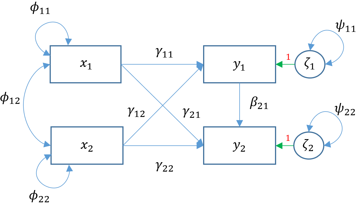
m4b <- '
  # regressions
    read ~ 1 + ppsych + motiv
    arith ~ 1 + motiv + read + ppsych
'
fit4b <- sem(m4b, data=dat)
summary(fit4b, fit.measures=TRUE)
The output is as follows:
  lavaan 0.6-7 ended normally after 15 iterations

  Estimator                                         ML
  Optimization method                           NLMINB
  Number of free parameters                          9

  Number of observations                           500

Model Test User Model:

  Test statistic                                 0.000
  Degrees of freedom                                 0

Parameter Estimates:

  Standard errors                             Standard
  Information                                 Expected
  Information saturated (h1) model          Structured

Regressions:
                   Estimate  Std.Err  z-value  P(>|z|)
  read ~
    ppsych           -0.275    0.037   -7.385    0.000
    motiv             0.461    0.037   12.404    0.000
  arith ~
    motiv             0.300    0.033    8.993    0.000
    read              0.597    0.035   17.004    0.000
    ppsych            0.068    0.031    2.212    0.027

Intercepts:
                   Estimate  Std.Err  z-value  P(>|z|)
   .read             -0.000    0.360   -0.000    1.000
   .arith             0.000    0.283    0.000    1.000

Variances:
                   Estimate  Std.Err  z-value  P(>|z|)
   .read             64.708    4.092   15.811    0.000
   .arith            39.923    2.525   15.811    0.000
The modification index is as follows:
modindices(fit4b,sort=TRUE)

[1] lhs      op       rhs      mi       epc      sepc.lv  sepc.all
[8] sepc.nox
<0 rows> (or 0-length row.names)
Quiz
Why is there no modification index left in fit4b? Is the chi-square you obtain the same or different from the modification index?
Answer: There is no modification index because it is a saturated model. The modification index is close to the Test User chi-square but slightly bigger since it is an approximation.
In Model 4B, we see that the degrees of freedom is zero which is what we expected from the modification index of 4.847. Recall that for Model 4A, the chi-square was 4.870 which is very close to our approximation. Additionally, the coefficient estimate is 0.068 which matches our modification index output exactly! In general, the modification index is just an approximation of the chi-square based on the Lagrange multiplier and may not match the results of actually re-running the model and obtaining the difference of the chi-square values. The degrees of freedom however, match what we expect, which is a one degree of freedom change resulting in our saturated path analysis model (Model 4B).
Model Test User Model: (Model 4A)

  Test statistic                                 4.870
  Degrees of freedom                                 1
  P-value (Chi-square)                           0.027

Model Test User Model: (Model 4B)

  Test statistic                                 0.000
  Degrees of freedom                                 0
Caveats of using modification indexes
Just because modification indexes present us with suggestions for improving our model fit does not mean as a researcher we can freely alter our model. Note that Type I error is the probability of finding a false positive, and altering our model based on modification indexes can have a grave impact on our Type I error. This means that you may be finding many statistically significant relationships that fail to be replicated in another sample. See our page on Retiring Statistical Significance for more information about the consequences of tweaking your hypothesis after your hypothesis has been made.
Model Fit Statistics
Modification indexes gives suggestions about ways to improve model fit, but it is helpful to assess the model fit of your current model to see if improvements are necessary. As we have seen, multivariate regression and path analysis models are not always saturated, meaning the degrees of freedom is not zero. This allows us to look at what are called Model Fit Statistics, which measure how closely the (population) model-implied covariance matrix $\Sigma{(\theta)}$ matches the (population) observed covariance matrix $\Sigma$. SEM is also known as covariance structure analysis, which means the hypothesis of interest is regarding the covariance matrix. The null and alternative hypotheses in an SEM model are
$$H_0: \Sigma{(\theta)}=\Sigma$$
$$H_1: \Sigma{(\theta)} \ne \Sigma$$
Typically, rejecting the null hypothesis is a good thing, but if we reject the SEM null hypothesis then we would reject our user model (which is bad). Failing to reject the model is good for our model because we have failed to disprove that our model is bad. Note that based on the logic of hypothesis testing, failing to reject the null hypothesis does not prove that our model is the true model, nor can we say it is the best model, as there may be many other competing models that can also fail to reject the null hypothesis. However, we can certainly say it isn’t a bad model, and it is the best model we can find at the moment. Think of a jury where it has failed to prove the criminal guilty, but it doesn’t necessarily mean he is innocent. Can you think of a famous person from the 90’s who fits this criteria?
Since we don’t have the population covariances to evaluate, they are estimated by the sample model-implied covariance $\Sigma(\hat{\theta})$ and sample covariance $S$. Then the difference $S-\Sigma(\hat{\theta})$ is a proxy for the fit of the model, and is defined as the residual covariance with values close to zero indicating that there is a relatively good fit.
Quiz
True or False. The residual covariance is defined as $\Sigma -\Sigma{(\theta)}$ and the closer this difference is to zero the better the fit.
Answer: False, the residual covariance uses sample estimates $S-\Sigma(\hat{\theta})$. Note that $\Sigma -\Sigma{(\theta)}=0$ is always true under the null hypothesis.
By default, lavaan outputs the model chi-square a.k.a Model Test User Model. To request additional fit statistics you add the fit.measures=TRUE option to summary, passing in the lavaan object fit4a.
#fit statistics
summary(fit4a, fit.measures=TRUE)

lavaan 0.6-7 ended normally after 14 iterations

  Estimator                                         ML
  Optimization method                           NLMINB
  Number of free parameters                          8

  Number of observations                           500

Model Test User Model:

  Test statistic                                 4.870
  Degrees of freedom                                 1
  P-value (Chi-square)                           0.027

Model Test Baseline Model:

  Test statistic                               674.748
  Degrees of freedom                                 5
  P-value                                        0.000

User Model versus Baseline Model:

  Comparative Fit Index (CFI)                    0.994
  Tucker-Lewis Index (TLI)                       0.971

Loglikelihood and Information Criteria:

  Loglikelihood user model (H0)              -3385.584
  Loglikelihood unrestricted model (H1)      -3383.149

  Akaike (AIC)                                6787.168
  Bayesian (BIC)                              6820.885
  Sample-size adjusted Bayesian (BIC)         6795.492

Root Mean Square Error of Approximation:

  RMSEA                                          0.088
  90 Percent confidence interval - lower         0.024
  90 Percent confidence interval - upper         0.172
  P-value RMSEA <= 0.05                          0.139

Standardized Root Mean Square Residual:

  SRMR                                           0.015
When fit measures are requested, lavaan outputs a plethora of statistics, but we will focus on the four commonly used ones:
- Model chi-square is the chi-square statistic we obtain from the maximum likelihood statistic (in lavaan, this is known as the Test Statistic for the Model Test User Model)
- CFI is the Comparative Fit Index – values can range between 0 and 1 (values greater than 0.90, conservatively 0.95 indicate good fit)
- TLI Tucker Lewis Index which also ranges between 0 and 1 (if it’s greater than 1 it should be rounded to 1) with values greater than 0.90 indicating good fit. If the CFI and TLI are less than one, the CFI is always greater than the TLI.
- RMSEA is the root mean square error of approximation
- In
lavaan, you also obtain a p-value of close fit, that the RMSEA < 0.05. If you reject the model, it means your model is not a close fitting model.
- In
Model chi-square
The model chi-square is defined as either $NF_{ML}$ or $(N-1)(F_{ML})$ depending on the statistical package where $N$ is the sample size and $F_{ML}$ is the fit function from maximum likelihood, which is a statistical method used to estimate the parameters in your model.
$$F_{ML} = \log |\hat{\Sigma}(\theta)| + tr(S {\hat{\Sigma}}^{-1}(\theta))-\log|S|-(p+q)$$
where $|\cdot|$ is the determinant of the matrix, $tr$ indicates the trace or the sum of the diagonal elements, $\log$ is the natural log, $p$ is the number of exogenous variables, and $q$ is the number of endogenous variables. Then depending on the software,
$$N F_{ML} \sim \chi^2(df_{User})$$
Since $df > 0$ the model chi-square $\chi^2(df_{\mbox{User}})$ is a meaningful test only when you have an over-identified model (i.e., there are still degrees of freedom left over after accounting for all the free parameters in your model).
Comparing the Model Test User Model for Model 4A (over-identified) model to the saturated Model 4B, we see that the Test Statistic degrees of freedom is zero for Model 4B, whereas Model 4A has 1 degree of freedom indicating an over-identified model. The Test Statistic is 4.870 and there is an additional row with P-value (Chi-square) of 0.027 indicating that we reject the null hypothesis.
The larger the chi-square value the larger the difference between the sample implied covariance matrix $\Sigma{(\hat{\theta})}$ and the sample observed covariance matrix $S$, and the more likely you will reject your model. We can recreate the p-value which is essentially zero, using the density function of the chi-square with 1 degrees of freedom $\chi^2_{1}=3.84$. Since $p < 0.05$, using the model chi-square criteria alone we reject the null hypothesis that the model fits the data. It is well documented in CFA and SEM literature that the chi-square is often overly sensitive in model testing especially for large samples. David Kenny states that for models with 75 to 200 cases chi-square is a reasonable measure of fit, but for 400 cases or more it is nearly almost always significant.
True or False. The larger the model chi-square test statistic, the larger the residual covariance $S-\hat{\Sigma}(\theta)$.
Answer: True. Since the model chi-square is proportional to the discrepancy of $S$ and $\Sigma{(\hat{\theta})}$, the higher the chi-square the more positive the value of $S-\Sigma{(\hat{\theta})}$, defined as residual covariance.
Our sample of $N=500$ is considered somewhat large, hence our conclusion may be supplemented with other fit indices.
#model chi-square
> pchisq(q=4.870,df=1,lower.tail=FALSE)
[1] 0.0273275
A note on sample size
Model chi-square is sensitive to large sample sizes, but does that mean we stick with small samples? The answer is no, larger samples are always preferred. CFA and the general class of structural equation model are actually large sample techniques and much of the theory is based on the premise that your sample size is as large as possible. So how big of a sample do we need? Kline (2016) notes the $N:q$ rule, which states that the sample size should be determined by the number of $q$ parameters in your model, and the recommended ratio is $20:1$. This means that if you have 10 parameters, you should have n=200. A sample size less than 100 is almost always untenable according to Kline.
The baseline model
The baseline model can be thought of as the “worst-fitting” model and simply assumes that there is absolutely no covariance between variables. Suppose we modified Model 4A to become a baseline model, we would take out all paths and covariances; essentially estimating only the variances. Since there is are no regression paths, there are no endogenous variables in our model and we would only have $x$’s and $\phi$’s.
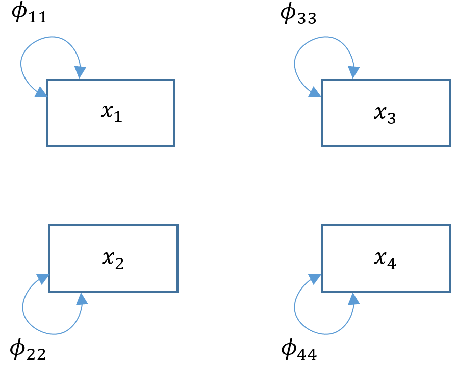
To model this in lavaan fit a model that simply estimates the variances of every variable in your model. For example read ~~ read estimates the exogenous variance of read ($\phi_{11}$).
m4c <- '
  # variances only
    read ~~ read
    ppsych ~~ ppsych
    motiv ~~ motiv
    arith ~~ arith
'
fit4c <- sem(m4c, data=dat)
summary(fit4c, fit.measures=TRUE)
To confirm whether we have truly generated the baseline model, we compare our model to the Model Test Baseline Model in lavaan. We see that the User Model chi-square is 707.017 with 6 degrees of freedom, which matches the Baseline Model chi-square. We will see in the next section how baseline models are used in testing model fit.
Model Test User Model:

  Test statistic                               707.017
  Degrees of freedom                                 6
  P-value (Chi-square)                           0.000

Model Test Baseline Model:

  Test statistic                               707.017
  Degrees of freedom                                 6
  P-value                                        0.000
Incremental versus absolute fit index
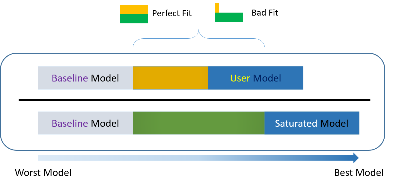
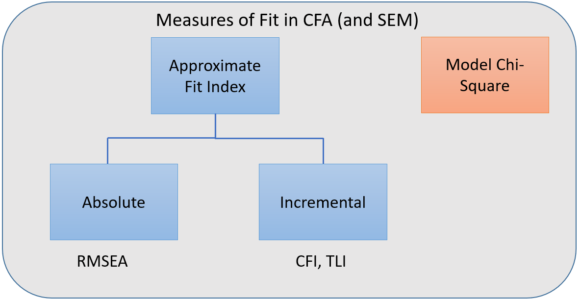
For over-identified models, there are many types of fit indexes available to the researcher. Historically, model chi-square was the only measure of fit but in practice the null hypothesis was often rejected due to the chi-square’s heightened sensitivity under large samples. To resolve this problem, approximate fit indexes that were not based on accepting or rejecting the null hypothesis were developed. Approximate fit indexes can be further classified into a) absolute and b) incremental or relative fit indexes. An incremental fit index (a.k.a. relative fit index) assesses the ratio of the deviation of the user model from the worst fitting model (a.k.a. the baseline model) against the deviation of the saturated model from the baseline model. Conceptually, if the deviation of the user model is the same as the deviation of the saturated model (a.k.a best fitting model), then the ratio should be 1. Alternatively, the more discrepant the two deviations, the closer the ratio is to 0 (see figure below). Examples of incremental fit indexes are the CFI and TLI.
An absolute fit index on the other hand, does not compare the user model against a baseline model, but instead compares it to the observed data. An example of an absolute fit index is the RMSEA (see flowchart below).
CFI (Comparative Fit Index)
The CFI or comparative fit index is a popular fit index as a supplement to the model chi-square. Let $\delta=\chi^2 – df$ where $df$ is the degrees of freedom for that particular model. The closer $\delta$ is to zero, the more the model fits the data. The formula for the CFI is:
$$CFI= \frac{\delta(\mbox{Baseline}) – \delta(\mbox{User})}{\delta(\mbox{Baseline})} $$
To manually calculate the CFI, recall the selected output from Model 4A model:
Model Test User Model:

  Test statistic                                 4.870
  Degrees of freedom                                 1
  P-value (Chi-square)                           0.027

Model Test Baseline Model:

  Test statistic                               674.748
  Degrees of freedom                                 5
  P-value                                        0.000
Then $\chi^2(\mbox{Baseline}) = 674.748$ and $df({\mbox{Baseline}}) = 5$, and $\chi^2(\mbox{User}) = 4.87$ and $df(\mbox{User}) = 1$. So $\delta(\mbox{Baseline}) = 674.748 – 4.87 = 669.878$ and $\delta(\mbox{User} )= 4.87 – 1=3.87$. We can plug all of this into the following equation:
$$CFI=\frac{669.878-3.87}{669.878}=0.994$$
Verify that the calculations match lavaan output. If $\delta(\mbox{User})=0$, then it means that the user model is not misspecified, so the numerator becomes $\delta(\mbox{Baseline})$ and the ratio becomes 1. The closer the CFI is to 1, the better the fit of the model; with the maximum being 1. Some criteria claims 0.90 to 0.95 as a good cutoff for good fit [citation needed].
TLI (Tucker Lewis Index)
The Tucker Lewis Index is also an incremental fit index that is commonly outputted with the CFI in popular packages such as Mplus and in this case lavaan. The term used in the TLI is the relative chi-square (a.k.a. normed chi-square) defined as $\frac{\chi^2}{df}$. Compared to the model chi-square, relative chi-square is less sensitive to sample size. To understand relative chi-square, we need to know that the expected value or mean of a chi-square is its degrees of freedom (i.e., $E(\chi^2(df)) = df$). For example, given that the test statistic truly came from a chi-square distribution with 4 degrees of freedom, we would expect the average chi-square value across repeated samples would also be 4. Suppose the chi-square from our data actually came from a distribution with 10 degrees of freedom but our model says it came from a chi-square with 4 degrees of freedom. Over repeated sampling, the relative chi-square would be $10/4=2.5$. Thus, $\chi^2/df = 1$ indicates perfect fit, and some researchers say that a relative chi-square greater than 2 indicates poor fit (Byrne,1989), other researchers recommend using a ratio as low as 2 or as high as 5 to indicate a reasonable fit (Marsh and Hocevar, 1985).
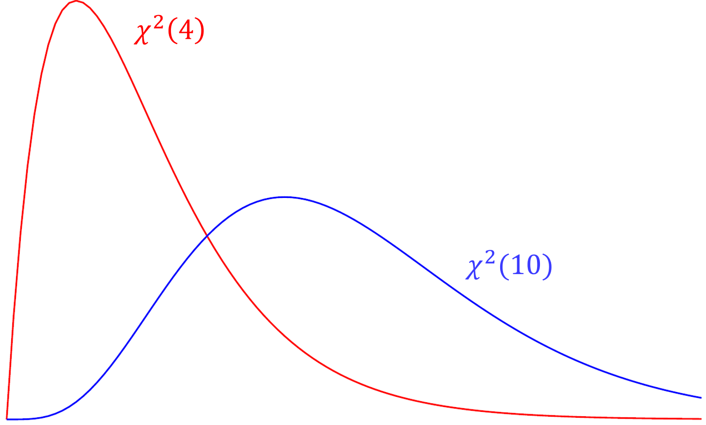
Quiz
Suppose you ran a CFA with 20 degrees of freedom. What would be the acceptable range of chi-square values based on the criteria that the relative chi-square greater than 2 indicates poor fit?
Answer
The range of acceptable chi-square values ranges between 20 (indicating perfect fit) and 40, since 40/20 = 2.
The TLI is defined as
$$TLI= \frac{\chi^2(\mbox{Baseline})/df(\mbox{Baseline})-\chi^2(\mbox{User})/df(\mbox{User})}{\chi^2(\mbox{Baseline})/df(\mbox{Baseline})-1}$$
Note that the TLI can be greater than 1 but for practical purposes we round it to 1. Given the eight-item one factor model:
$$TLI= \frac{674.748/5-4.870/1}{674.748/5-1} =\frac{130.0796}{133.9496}=0.971.$$
We can confirm our answers for both the TLI and CFI which are reported together in lavaan
User Model versus Baseline Model:

  Comparative Fit Index (CFI)                    0.994
  Tucker-Lewis Index (TLI)                       0.971
You can think of the TLI as the ratio of the deviation of the null (baseline) model from user model to the deviation of the baseline (or null) model to the perfect fit model $\chi^2/df = 1$. The more similar the deviation from the baseline model, the closer the ratio to one. A perfect fitting model which generate a TLI which equals 1. David Kenny states that if the CFI is less than one, then the CFI is always greater than the TLI. CFI pays a penalty of one for every parameter estimated. Because the TLI and CFI are highly correlated, only one of the two should be reported.
RMSEA
The root mean square error of approximation is an absolute measure of fit because it does not compare the discrepancy of the user model relative to a baseline model like the CFI or TLI. Instead, RMSEA defines $\delta$ as the non-centrality parameter which measures the degree of misspecification. Recall from the CFI that $\delta=\chi^2 – df$ where $df$ is the degrees of freedom for that particular model. The greater the $\delta$ the more misspecified the model.
$$ RMSEA = \sqrt{\frac{\delta}{df(N-1)}} $$
where $N$ is the total number of observations. The cutoff criteria as defined in Kline (2016, p.274-275)
- $\le 0.05$ (close-fit)
- between $.05$ and $.08$ (reasonable approximate fit, fails close-fit but also fails poor-fit)
- $>= 0.10$ (poor-fit)
In Model 4A, $N=500$, $df(\mbox{User}) = 1$ and $\delta(\mbox{User} )= 4.87 – 1=3.87$ which we already known from calculating the CFI. Here $\delta$ is about 4 times the degrees of freedom.
$$ RMSEA = \sqrt{\frac{3.87}{1(499)}} = \sqrt{0.007755511}=0.088$$
Our RMSEA = 0.088 indicating reasonable approximate fit, as evidence by the large $\delta(\mbox{User} )$ relative to the degrees of freedom.
  Number of observations                           500

<... output omitted ...>

Root Mean Square Error of Approximation:

  RMSEA                                          0.088
  90 Percent confidence interval - lower         0.024
  90 Percent confidence interval - upper         0.172
  P-value RMSEA <= 0.05                          0.139
Given that the p-value of the model chi-square was less than 0.05, the CFI = 0.994 and the RMSEA = 0.088, and looking at the standardized loadings we report to the Principal Investigator that Model 4A is a reasonable model.
The Measurement Model
We have talked so far about how to model structural relationships between observed variables. A measurement model is essentially a multivariate regression model where the predictor is an exogenous or endogenous latent variable (a.k.a factor). The model is defined as
$$\mathbf{x= \tau_x + \Lambda_x \xi+ \delta}$$
Definitions
- $\mathbf{x} =(x_1, \cdots, x_q)’$ vector of $x$-side indicators
- $\mathbf{\tau_x}$ vector of $q$ intercepts for $x$-side indicators
- $\mathbf{\xi}$ vector of $n$ latent exogenous variables
- $\mathbf{\delta}= ( \delta_1, \cdots, \delta_q)’$ vector of residuals for $x$-side indicators
- $\mathbf{\Lambda_x}$ matrix of loadings ($q \times n$) corresponding to the latent exogenous variables
- $\mathbf{\theta_{\delta}}$ variance or covariance of residuals for $x$-side indicators
The term $\tau_{x_{1}}$ means the intercept of the first item, and $\lambda^x_2$ is the loading of the second item with the factor and $\epsilon_{3}$ is the residual of the third item, after accounting for the only factor.
Suppose we have three outcomes or $x$-side indicators ($x_1,x_2,x_3$) measured by a single latent exogenous variable $\xi$. Then the path diagram (Model 5A) for our factor model looks like the following. Take note that the intercepts $\mathbf{\tau_x}$ are not shown but still modeled, and that the measurement arrows are pointing to the left. 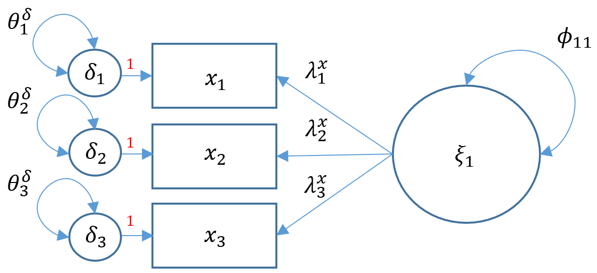
True or False. $\xi$ variables do not have residual covariances
Answer: True. $\xi$ are latent exogenous variables which do not have residuals hence no residual covariances
True or False. $x_i$ variables do not have residual covariances
Answer: False. $x_i$’s are manifest exogenous variables but in fact are explained by the latent exogenous variable, therefore it has a residual term and residual variance (unexplained variance), most notably $\theta_{\delta}$.
Identification of a three-item factor analysis
Identification of the one factor model with three items is necessary due to the fact that we have 7 parameters from the model-implied covariance matrix $\Sigma(\theta)$ (e.g., three factor loadings, three residual variances and one factor variance) but only $3(4)/2=6$ known values to work with. The extra parameter comes from the fact that we do not observe the factor but are estimating its variance. In order to identify a factor model with three or more items, there are two options known as the marker method and the variance standardization method. The
- marker method fixes the first loading of each factor to 1,
- variance standardization method fixes the variance of each factor to 1 but freely estimates all loadings.
In matrix notation, the marker method (Option 1) can be shown as
$$
\Sigma(\theta)=
\phi_{11}
\begin{pmatrix}
1 \\
\lambda^{x}_{2} \\
\lambda^{x}_{3}
\end{pmatrix}
\begin{pmatrix}
1 & \lambda^{x}_{2} & \lambda^{x}_{3} \\
\end{pmatrix}
+
\begin{pmatrix}
\theta^{\delta}_{11} & 0 & 0 \\
0 & \theta^{\delta}_{22} & 0 \\
0 & 0 & \theta^{\delta}_{33} \\
\end{pmatrix}
$$
In matrix notation, the variance standardization method (Option 2) looks like
$$
\Sigma(\theta)=
(1)
\begin{pmatrix}
\lambda^{x}_{1} \\
\lambda^{x}_{2} \\
\lambda^{x}_{3}
\end{pmatrix}
\begin{pmatrix}
\lambda^{x}_{1} & \lambda^{x}_{2} & \lambda^{x}_{3} \\
\end{pmatrix}
+
\begin{pmatrix}
\theta^{\delta}_{11} & 0 & 0 \\
0 & \theta^{\delta}_{22} & 0 \\
0 & 0 & \theta^{\delta}_{33} \\
\end{pmatrix}
$$
Notice in both models that the residual covariances stay freely estimated.
Exercise
For the variance standardization method, go through the process of calculating the degrees of freedom. If we have six known values is this model just-identified, over-identified or under-identified?
Answer: We start with 10 unique parameters in the model-implied covariance matrix. Since we fix one factor variance, and 3 unique residual covariances, the number of free parameters is $10-(1+3)=6$. Since we have 6 known values, our degrees of freedom is $6-6=0$, which is defined to be saturated.
Exogenous factor analysis (Model 5A)
Let’s see how we can run a one-factor measurement in lavaan with Verbal IQ verbal, SES ses and Negative Parental Psychology ppsych as indicators of the factor (latent exogenous variable) Risk risk.
m5a <- 'risk =~ verbal + ses + ppsych
#intercepts (nu = tau)
verbal ~ 1
ses ~ 1
ppsych ~ 1'
fit5a <- sem(m5a, data=dat)
summary(fit5a, standardized=TRUE)
The first line is the model statement. Recall that =~ represents the indicator equation where the latent variable is on the left and the indicators (or observed variables) are to the right the symbol. Here we name our factor risk, which is indicated by verbal, ses and ppsych (note the names must match the variable names in the dataset). Here we explicitly model the intercepts of the indicators using verbal ~ 1, ses ~ 1 and ppsych ~ 1. Then store the model into object m5a for Model 5A. The second line is where we specify that we want to run the analysis using the sem function, which is actually a wrapper for the lavaan function. The model to be estimated is m5a and the dataset to be used is dat; storing the output into object fit5a. Finally summary(fit5a, standardized=TRUE) requests a summary of the analysis, outputting the estimator used, the number of free parameters, the test statistic, estimated means, standardized loadings and standardized variances.
lavaan 0.6-7 ended normally after 37 iterations

  Estimator                                         ML
  Optimization method                           NLMINB
  Number of free parameters                          9

  Number of observations                           500

Model Test User Model:

  Test statistic                                 0.000
  Degrees of freedom                                 0

Parameter Estimates:

  Standard errors                             Standard
  Information                                 Expected
  Information saturated (h1) model          Structured

Latent Variables:
                   Estimate  Std.Err  z-value  P(>|z|)   Std.lv  Std.all
  risk =~
    verbal            1.000                               6.166    0.617
    ses               1.050    0.126    8.358    0.000    6.474    0.648
    ppsych           -1.050    0.126   -8.358    0.000   -6.474   -0.648

Intercepts:
                   Estimate  Std.Err  z-value  P(>|z|)   Std.lv  Std.all
   .verbal            0.000    0.447    0.000    1.000    0.000    0.000
   .ses              -0.000    0.447   -0.000    1.000   -0.000   -0.000
   .ppsych           -0.000    0.447   -0.000    1.000   -0.000   -0.000
    risk              0.000                               0.000    0.000

Variances:
                   Estimate  Std.Err  z-value  P(>|z|)   Std.lv  Std.all
   .verbal           61.781    5.810   10.634    0.000   61.781    0.619
   .ses              57.884    5.989    9.664    0.000   57.884    0.580
   .ppsych           57.884    5.989    9.664    0.000   57.884    0.580
    risk             38.019    6.562    5.794    0.000    1.000    1.000
By default, lavaan chooses the marker method (Option 1) if nothing else is specified. To better interpret the factor loadings, often times you would request the standardized solutions. Notice two additional columns in the output, Std.lv and Std.all. For users of Mplus, Std.lv corresponds to STD and Std.all corresponds to STDYX. In the variance standardization method Std.lv, we only standardize by the predictor (the factor, X). Std.all not only standardizes by the variance of the latent variable ($\xi$) and also by the variance of outcome which in this case are the indicators $x$.
Exercise
Try to fit the model using variance standardization method.
Answer: : Refer to Running a one-factor CFA in lavaan for more details on how perform variance standardization in lavaan.
A note on endogenous measurement models (Model 5B)
Not all latent variables are exogenous. If in the case that the latent variable is endogenous we will rename the factor $\eta$.
Suppose again that we have three items except now they are labeled ($y_1,y_2,y_3$). For a latent endogenous variable, the structure of the measurement model remains the same except now the parameters are re-labeled as $y$-side variables. The path diagram for Model 5B is shown below (note, intercepts $\mathbf{\tau_y}$ are not shown but still implicitly modeled):

Note that the direction of the arrows face the right. In LISREL path diagram notation, exogenous latent variables have measurement arrows pointing to the left and endogenous latent variables have measurement arrows pointing to the right. Exogenous latent variables correspond to x-side models and endogenous latent variables to y-side models. Here the $y$-side measurement model is defined as
$$\mathbf{y= \tau_y + \Lambda_y \eta + \epsilon}$$
Definitions
- $\mathbf{y} = (y_1, \cdots, y_p)’$ vector of $y$-side indicators
- $\mathbf{\tau_y}$ vector of $p$ intercepts for $y$-side indicators
- $\mathbf{\eta}$ vector of $m$ latent endogenous variables
- $\mathbf{\epsilon}= ( \epsilon_1, \cdots, \epsilon_p)’$ vector of residuals for $y$-side indicators
- $\mathbf{\Lambda_y}$ matrix of loadings ($m \times q$) corresponding to the latent endogenous variables
- $\mathbf{\theta_{\epsilon}}$ variance or covariance of residuals for $y$-side indicators
The main difference between Models 5A and 5B are simply that Model 5A is an exogenous latent factor analysis whereas Model 5B is an endogenous latent factor analysis, meaning that it is being predicted by another latent variable. Since we currently have no predictors of $\eta_1$, this is just a hypothetical model. In the section below on structural regression, we will see an endogenous latent variable modeled with real-world data. Exogenous latent measurement models are what are classified as x-side variables which point to the left in a path diagram and endogenous latent measurement models are known as y-side latent variables which point to the right in a path diagram.
Up to this point we have studied multivariate measurement models that define the relationship between indicators and latent variables, as well as multivariate regression and path models that define the causal relationship between observed endogenous and exogenous variables. In the next section, we will see how structural regression models allows us to model relationships between exogenous and endogenous latent variables.
True or False. In a LISREL path diagram, endogenous latent variables have right-pointing arrows to the indicators.
Answer: True. The indicators and latent endogenous variable is known as $y$-side variables.
The Structural Model
Structural Regression Model
So far we have discussed all the individual components that make up the structural regression model. Recall that multivariate regression involves regression with simultaneous endogenous variables and path analysis allows for explanatory endogenous variables. Confirmatory factor analysis is a measurement model that links latent variables to indicators. Finally, structural regression unifies the measurement and structural models to allow for explanatory latent variables, whether endogenous or exogenous.
$$\mathbf{x= \tau_x + \Lambda_x \xi+ \delta}$$
$$\mathbf{y= \tau_y + \Lambda_y \eta + \epsilon}$$
$$\mathbf{\eta = \alpha + B \eta + \Gamma \xi + \zeta}$$
Definitions
Measurement variables
- $\mathbf{x} = (x_1, \cdots, x_q)’$ vector of $x$-side indicators
- $\mathbf{y} = (y_1, \cdots, y_p)’$ vector of $y$-side indicators
- $\mathbf{\tau_x}$ vector of $q$ intercept terms for $x$-side indicators
- $\mathbf{\tau_y}$ vector of $p$ intercept terms for $y$-side indicators
- $\mathbf{\xi}$ vector of $n$ latent exogenous variables
- $\mathbf{\eta}$ vector of $m$ latent endogenous variables
- $\mathbf{\delta}= ( \delta_1, \cdots, \delta_q)’$ vector of residuals for $x$-side indicators
- $\mathbf{\epsilon}= ( \epsilon_1, \cdots, \epsilon_p)’$ vector of residuals for $y$-side indicators
- $\mathbf{\Lambda_x}$ matrix of loadings ($q \times n$) corresponding to the latent exogenous variables
- $\mathbf{\Lambda_y}$ matrix of loadings ($p \times m$) corresponding to the latent endogenous variables
- $\mathbf{\theta_{\delta}}$ variance or covariance of residuals for $x$-side indicators
- $\mathbf{\theta_{\epsilon}}$ variance or covariance of residuals for $y$-side indicators
Structural variables
- $\mathbf{\alpha}$ a vector of $m$ intercepts
- $\Gamma$ a matrix of regression coefficients ($m \times n$) of latent exogenous to latent endogenous variables whose $i$-th row indicates the latent endogenous variable and $j$-th column indicates the latent exogenous variable
- $B$ a matrix of regression coefficients ($m \times m$) of latent endogenous to latent endogenous variables whose $i$-th row indicates the target endogenous variable and $j$-th column indicates the source endogenous variable.
- $\zeta= ( \zeta_1, \cdots, \zeta_m)’$ vector of residuals for the latent endogenous variable
Assumptions
- $\eta$ and $\xi$ are not observed
- $\epsilon$ and $\delta$ are errors of measurement for $y$ and $x$ respectively
- $\epsilon$ is uncorrelated with $\delta$
To specify the full structural regression model, it is more intuitive to start with the measurement model and then specify how the latent variables relate to each other (the structural model). In order for latent exogenous variables to explain latent endogenous variables, two separate measurement models must be established.
First let’s specify the latent exogenous measurement model with six items where the first three $x$-side indicators ($x_1, x_2, x_3$) are measured by $\xi_1$ and the latter three ($x_4,x_5,x_6$) are measured by $\xi_2$. The un-identified measurement model for two latent exogenous variables with three indicators each is:
$$
\begin{pmatrix}
x_{1} \\
x_{2} \\
x_{3} \\
x_{4} \\
x_{5} \\
x_{6} \\
\end{pmatrix}
=
\begin{pmatrix}
\tau_{x_{1}} \\
\tau_{x_{2}} \\
\tau_{x_{3}} \\
\tau_{x_{4}} \\
\tau_{x_{5}} \\
\tau_{x_{6}}
\end{pmatrix}
+
\begin{pmatrix}
\lambda^{x}_{11} & \lambda^{x}_{12} \\
\lambda^{x}_{21} & \lambda^{x}_{22} \\
\lambda^{x}_{31} & \lambda^{x}_{32} \\
\lambda^{x}_{41} & \lambda^{x}_{42} \\
\lambda^{x}_{51} & \lambda^{x}_{52} \\
\lambda^{x}_{61} & \lambda^{x}_{62}
\end{pmatrix}
\begin{pmatrix}
\xi_{1} \\
\xi_{2}
\end{pmatrix}
+
\begin{pmatrix}
\delta_{1} \\
\delta_{2} \\
\delta_{3} \\
\delta_{4} \\
\delta_{5} \\
\delta_{6}
\end{pmatrix}
$$
Now that we’ve established the exogenous measurement model, let’s move to the endogenous measurement model. The three $y$-side indicators $y_1, y_2, y_3$ are measured by one factor $\eta_1$.
$$
\begin{pmatrix}
y_{1} \\
y_{2} \\
y_{3}
\end{pmatrix}
=
\begin{pmatrix}
\tau_{y_{1}} \\
\tau_{y_{2}} \\
\tau_{y_{3}}
\end{pmatrix}
+
\begin{pmatrix}
\lambda^{y}_{11} \\
\lambda^{y}_{21} \\
\lambda^{y}_{31}
\end{pmatrix}
\begin{pmatrix}
\eta_{1}
\end{pmatrix}
+
\begin{pmatrix}
\epsilon_{1}\\
\epsilon_{2} \\
\epsilon_{3}
\end{pmatrix}
$$
Now that we’ve established both $x$-side and $y$-side measurement models, we can specify the structural model.
Structural regression with one endogenous variable (Model 6A)
Just as the structural model in multivariate regression and path analysis specifies relationships among observed variables, structural regression specifies the relationship between latent variables. In Model 6A, we have two latent exogenous variables ($\xi_1, \xi_2$) predicting one latent endogenous variable ($\eta_1$).
$$
\eta_{1}
=
\alpha_1
+
\begin{pmatrix}
\gamma_{11} & \gamma_{12}
\end{pmatrix}
\begin{pmatrix}
\xi_1 \\
\xi_2
\end{pmatrix}
+
0 \cdot \eta_1
+
\zeta_{1}
$$
Recall that the $\Gamma$ matrix specifies the relationship between exogenous and endogenous variables, so that $\gamma_{11}$ is the regression path of the first endogenous variable $\eta_1$ with the first exogenous variable $\xi_1$ and $\gamma_{12}$ is the regression path of $\eta_1$ with the second exogenous variable $\xi_2$. Since there are no endogenous variables predicting each other, $B=0$.
True or False. In Model 6A, $B=0$ here implies that there are no structural paths.
Answer: False. $B=0$ means that there are no endogenous variables predicting each other as in path analysis, but $\Gamma$ defines the structural paths between exogenous and endogenous variables.
True or False. $\eta = \eta_1$ because there is only endogenous variable, however $\Gamma$ is a $1 \times 2$ matrix because there are two exogenous variables.
Answer: True. The number of rows in $\eta$ tells you how many endogenous variables. Here there is only one outcome regardless the number of exogenous predictors.
True or False. You can simplify Model 6A model to the path analysis model by removing the two measurement models.
Answer: False (somewhat). Even if you remove the measurement models you still have the equation $\mathbf{\eta = \alpha + \Gamma \xi + B \eta + \zeta}$ which is defined only for latent endogenous variables. However, simply exchange $y$ for $\eta$ and $x$ for $\xi$ and you will obtain the path analysis model.
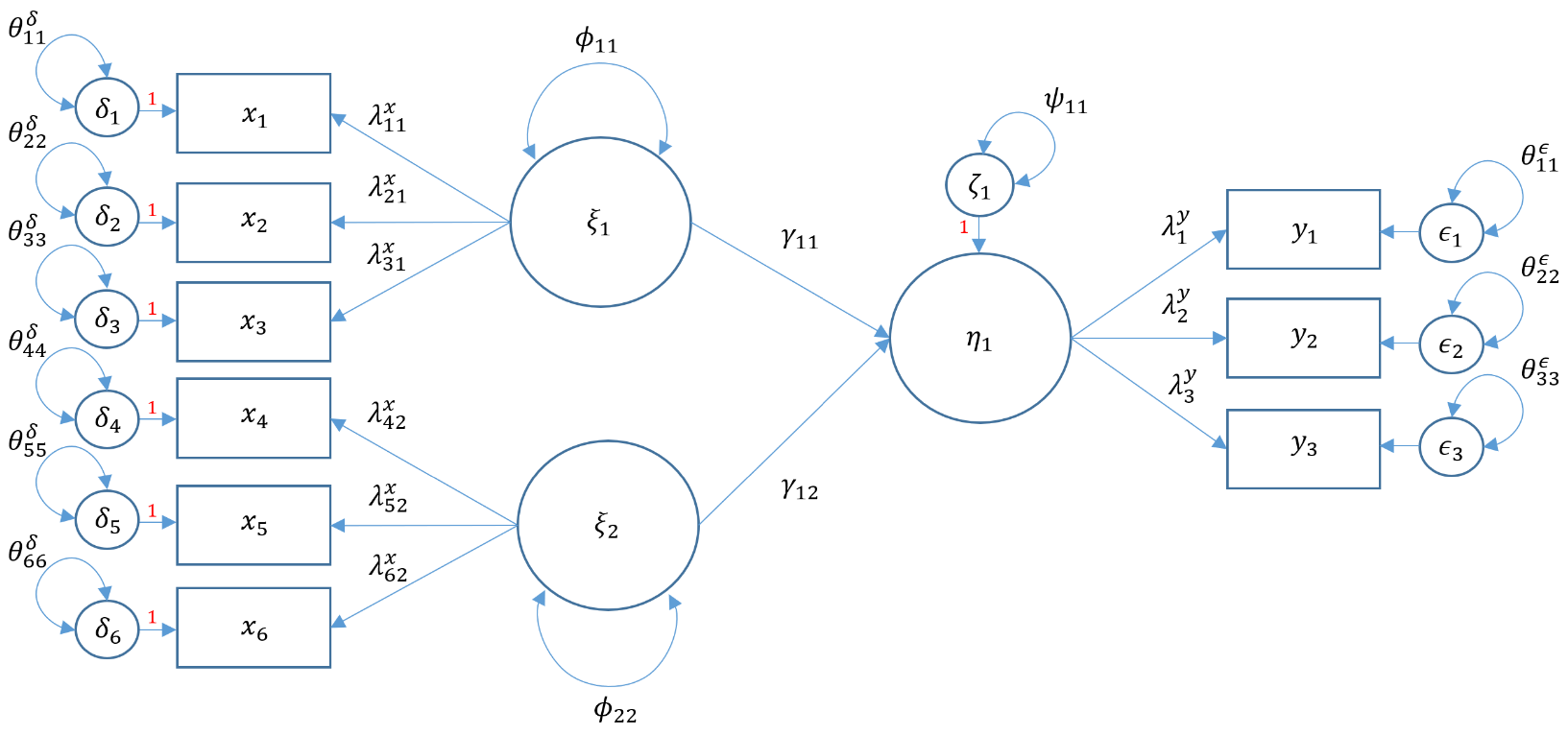
Let’s use lavaan to implement Model 6A with our dataset. First, establish the measurement model and proceed to the structural. Adjustment is the first latent exogenous variable $\xi_1$ consisting of three $x$-side indicators – Motivation, Harmony and Stability, adjust =~ motiv + harm + stabi. Risk is the second latent exogenous variable $\xi_2$ with three $x$-side indicators, Verbal IQ, Negative Parental Psychology and SES risk =~ verbal + ppsych + ses. Then proceed to the only endogenous variable, Achievement ($\eta_1$) with three $y$-side indicators Reading, Arithmetic and Spelling achieve =~ read + arith + spell. Finally, let’s establish the structural regression. We hypothesize that Adjustment positively predicts and Risk negatively predicts student Achievement and in lavaan we specify achieve ~ adjust + risk. Note that we do not explicitly model the intercepts for our latent regressions. (How would you explicitly model them?)
m6a <- '
# measurement model
adjust =~ motiv + harm + stabi
risk =~ verbal + ppsych + ses
achieve =~ read + arith + spell
# regressions
achieve ~ adjust + risk
'
fit6a <- sem(m6a, data=dat)
summary(fit6a, standardized=TRUE, fit.measures=TRUE)
The output is as follows:
lavaan 0.6-7 ended normally after 130 iterations

  Estimator                                         ML
  Optimization method                           NLMINB
  Number of free parameters                         21

  Number of observations                           500

Model Test User Model:

  Test statistic                               148.982
  Degrees of freedom                                24
  P-value (Chi-square)                           0.000

Model Test Baseline Model:

  Test statistic                              2597.972
  Degrees of freedom                                36
  P-value                                        0.000

User Model versus Baseline Model:

  Comparative Fit Index (CFI)                    0.951
  Tucker-Lewis Index (TLI)                       0.927

Loglikelihood and Information Criteria:

  Loglikelihood user model (H0)             -15517.857
  Loglikelihood unrestricted model (H1)     -15443.366

  Akaike (AIC)                               31077.713
  Bayesian (BIC)                             31166.220
  Sample-size adjusted Bayesian (BIC)        31099.565

Root Mean Square Error of Approximation:

  RMSEA                                          0.102
  90 Percent confidence interval - lower         0.087
  90 Percent confidence interval - upper         0.118
  P-value RMSEA <= 0.05                          0.000

Standardized Root Mean Square Residual:

  SRMR                                           0.041

Parameter Estimates:

  Standard errors                             Standard
  Information                                 Expected
  Information saturated (h1) model          Structured

Latent Variables:
                   Estimate  Std.Err  z-value  P(>|z|)   Std.lv  Std.all
  adjust =~
    motiv             1.000                               9.324    0.933
    harm              0.884    0.041   21.774    0.000    8.246    0.825
    stabi             0.695    0.043   15.987    0.000    6.478    0.648
  risk =~
    verbal            1.000                               7.319    0.733
    ppsych           -0.770    0.075  -10.223    0.000   -5.636   -0.564
    ses               0.807    0.076   10.607    0.000    5.906    0.591
  achieve =~
    read              1.000                               9.404    0.941
    arith             0.837    0.034   24.437    0.000    7.873    0.788
    spell             0.976    0.028   34.338    0.000    9.178    0.919

Regressions:
                   Estimate  Std.Err  z-value  P(>|z|)   Std.lv  Std.all
  achieve ~
    adjust            0.375    0.046    8.085    0.000    0.372    0.372
    risk              0.724    0.078    9.253    0.000    0.564    0.564

Covariances:
                   Estimate  Std.Err  z-value  P(>|z|)   Std.lv  Std.all
  adjust ~~
    risk             32.098    4.320    7.431    0.000    0.470    0.470

Variances:
                   Estimate  Std.Err  z-value  P(>|z|)   Std.lv  Std.all
   .motiv            12.870    2.852    4.512    0.000   12.870    0.129
   .harm             31.805    2.973   10.698    0.000   31.805    0.319
   .stabi            57.836    3.990   14.494    0.000   57.836    0.580
   .verbal           46.239    4.788    9.658    0.000   46.239    0.463
   .ppsych           68.033    5.068   13.425    0.000   68.033    0.682
   .ses              64.916    4.975   13.048    0.000   64.916    0.650
   .read             11.372    1.608    7.074    0.000   11.372    0.114
   .arith            37.818    2.680   14.109    0.000   37.818    0.379
   .spell            15.560    1.699    9.160    0.000   15.560    0.156
    adjust           86.930    6.830   12.727    0.000    1.000    1.000
    risk             53.561    6.757    7.927    0.000    1.000    1.000
   .achieve          30.685    3.449    8.896    0.000    0.347    0.347
Structural regression with two endogenous variables (Model 6B)
Suppose we want to consider a single exogenous latent variable $\xi_1$ predicting two endogenous latent variables $\eta_1, \eta_2$ and additionally that one of the endogenous variables predicts another. What additional matrix do you think we need? Since we have already established the measurement model in 6A we can re-use the specification, making note that the measurement model now has one $x$-side model and two $y$-side models. However, not only do we need $\Gamma$ to model the relationship of the exogenous variable to the two endogenous variables, we need the $B$ matrix to specify the relationship of the first endogenous variable to the other.
$$
\begin{pmatrix}
\eta_{1} \\
\eta_{2}
\end{pmatrix}
=
\begin{pmatrix}
\alpha_1 \\
\alpha_2
\end{pmatrix}
+
\begin{pmatrix}
\gamma_{11}\\
\gamma_{21}
\end{pmatrix}
\xi_1
+
\begin{pmatrix}
0 & 0\\
\beta_{21} & 0
\end{pmatrix}
\begin{pmatrix}
\eta_1 \\
\eta_2
\end{pmatrix}
+
\begin{pmatrix}
\zeta_{1}\\
\zeta_{2}
\end{pmatrix}
$$
Writing out the equations we get:
$$
\eta_{1}
=
\alpha_1
+
\gamma_{11} \xi_1
+
\zeta_{1}
$$
$$
\eta_{2}
=
\alpha_2
+
\gamma_{21} \xi_1
+
\beta_{21} \eta_1
+
\zeta_{2}
$$
The first equation specifies that the first endogenous variable is being predicted only by the exogenous variable whereas the second equation specifies that the second endogenous variable is being predicted by both the exogenous variable and first endogenous variable.
True or False. The diagonal entries of $B$ are always zero.
Answer: True. You cannot have a variable predict itself so $\beta_{11}=\beta_{22}=0$.
True or False. $\beta_{21}$ means that the second endogenous variable is predicting the first endogenous variable.
Answer: True.
True or False. $\gamma_{21}$ means that the second exogenous variable is predicting the first endogenous variable.
Answer: False. The first index specifies the endogenous variable, so $\gamma_{21}$ means the first exogenous variable predicts first endogenous variable (read it “backwards”). Since we only have one $\xi$ you can remove the second index and just say $\gamma_2$.
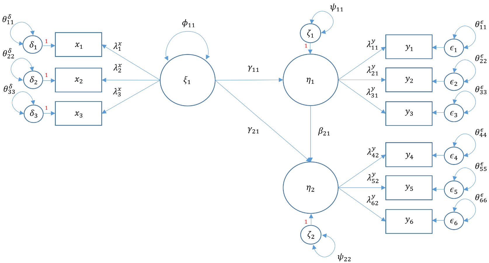
Since lavaan uses what are known as all $y$-side models, there is no need to different between exogenous and endogenous latent variables. As such, the measurement model in 6B is exactly the same as in Model 6A. The only modification then is the structural regression. We hypothesize that Risk negatively predicts Adjustment adjust ~ risk and that Adjustment (an endogenous variable) and Risk (an exogenous variable) predict Achievement achieve ~ adjust + risk.
m6b <- '
# measurement model
adjust =~ motiv + harm + stabi
risk =~ verbal + ses + ppsych
achieve =~ read + arith + spell
# regressions
adjust ~ risk
achieve ~ adjust + risk
'
fit6b <- sem(m6b, data=dat)
summary(fit6b, standardized=TRUE, fit.measures=TRUE)
The output is as follows:
lavaan 0.6-7 ended normally after 112 iterations

  Estimator                                         ML
  Optimization method                           NLMINB
  Number of free parameters                         21

  Number of observations                           500

Model Test User Model:

  Test statistic                               148.982
  Degrees of freedom                                24
  P-value (Chi-square)                           0.000

Model Test Baseline Model:

  Test statistic                              2597.972
  Degrees of freedom                                36
  P-value                                        0.000

User Model versus Baseline Model:

  Comparative Fit Index (CFI)                    0.951
  Tucker-Lewis Index (TLI)                       0.927

Loglikelihood and Information Criteria:

  Loglikelihood user model (H0)             -15517.857
  Loglikelihood unrestricted model (H1)     -15443.366

  Akaike (AIC)                               31077.713
  Bayesian (BIC)                             31166.220
  Sample-size adjusted Bayesian (BIC)        31099.565

Root Mean Square Error of Approximation:

  RMSEA                                          0.102
  90 Percent confidence interval - lower         0.087
  90 Percent confidence interval - upper         0.118
  P-value RMSEA <= 0.05                          0.000

Standardized Root Mean Square Residual:

  SRMR                                           0.041

Parameter Estimates:

  Standard errors                             Standard
  Information                                 Expected
  Information saturated (h1) model          Structured

Latent Variables:
                   Estimate  Std.Err  z-value  P(>|z|)   Std.lv  Std.all
  adjust =~
    motiv             1.000                               9.324    0.933
    harm              0.884    0.041   21.774    0.000    8.246    0.825
    stabi             0.695    0.043   15.987    0.000    6.478    0.648
  risk =~
    verbal            1.000                               7.319    0.733
    ses               0.807    0.076   10.607    0.000    5.906    0.591
    ppsych           -0.770    0.075  -10.223    0.000   -5.636   -0.564
  achieve =~
    read              1.000                               9.404    0.941
    arith             0.837    0.034   24.437    0.000    7.873    0.788
    spell             0.976    0.028   34.338    0.000    9.178    0.919

Regressions:
                   Estimate  Std.Err  z-value  P(>|z|)   Std.lv  Std.all
  adjust ~
    risk              0.599    0.076    7.837    0.000    0.470    0.470
  achieve ~
    adjust            0.375    0.046    8.085    0.000    0.372    0.372
    risk              0.724    0.078    9.253    0.000    0.564    0.564

Variances:
                   Estimate  Std.Err  z-value  P(>|z|)   Std.lv  Std.all
   .motiv            12.870    2.852    4.512    0.000   12.870    0.129
   .harm             31.805    2.973   10.698    0.000   31.805    0.319
   .stabi            57.836    3.990   14.494    0.000   57.836    0.580
   .verbal           46.239    4.788    9.658    0.000   46.239    0.463
   .ses              64.916    4.975   13.048    0.000   64.916    0.650
   .ppsych           68.033    5.068   13.425    0.000   68.033    0.682
   .read             11.372    1.608    7.074    0.000   11.372    0.114
   .arith            37.818    2.680   14.109    0.000   37.818    0.379
   .spell            15.560    1.699    9.160    0.000   15.560    0.156
   .adjust           67.694    6.066   11.160    0.000    0.779    0.779
    risk             53.561    6.757    7.927    0.000    1.000    1.000
   .achieve          30.685    3.449    8.896    0.000    0.347    0.347
Structural regression with an observed endogenous variable (Model 6C)
Structural models relate latent to latent variables. Suppose you wanted to look at how Risk or Adjustment relate in particular to Reading scores rather than overall student achievement. In LISREL notation, the matrices $\Gamma$ or $B$ in the structural regression allow only for relationships among latent variables. However, lavaan and other software programs such as Mplus allow the user to easily specify the relationship between an observed and latent variable. The code is as easy as specifying read ~ adjust + risk where adjust and risk are latent variables.
#structural regression model C indicator DV
m6c <- '
# measurement model
adjust =~ motiv + harm + stabi
risk =~ verbal + ses + ppsych
# regressions
adjust ~ risk
read ~ adjust + risk
'
fit6c <- sem(m6c, data=dat)
summary(fit6c, standardized=TRUE, fit.measures=TRUE)
The output is as follows:
lavaan 0.6-7 ended normally after 105 iterations

  Estimator                                         ML
  Optimization method                           NLMINB
  Number of free parameters                         16

  Number of observations                           500

Model Test User Model:

  Test statistic                                35.555
  Degrees of freedom                                12
  P-value (Chi-square)                           0.000

Model Test Baseline Model:

  Test statistic                              1339.008
  Degrees of freedom                                21
  P-value                                        0.000

User Model versus Baseline Model:

  Comparative Fit Index (CFI)                    0.982
  Tucker-Lewis Index (TLI)                       0.969

Loglikelihood and Information Criteria:

  Loglikelihood user model (H0)             -12370.103
  Loglikelihood unrestricted model (H1)     -12352.325

  Akaike (AIC)                               24772.206
  Bayesian (BIC)                             24839.640
  Sample-size adjusted Bayesian (BIC)        24788.855

Root Mean Square Error of Approximation:

  RMSEA                                          0.063
  90 Percent confidence interval - lower         0.039
  90 Percent confidence interval - upper         0.087
  P-value RMSEA <= 0.05                          0.170

Standardized Root Mean Square Residual:

  SRMR                                           0.025

Parameter Estimates:

  Standard errors                             Standard
  Information                                 Expected
  Information saturated (h1) model          Structured

Latent Variables:
                   Estimate  Std.Err  z-value  P(>|z|)   Std.lv  Std.all
  adjust =~
    motiv             1.000                               9.172    0.918
    harm              0.914    0.043   21.334    0.000    8.379    0.839
    stabi             0.716    0.045   16.025    0.000    6.569    0.658
  risk =~
    verbal            1.000                               7.208    0.722
    ses               0.829    0.076   10.848    0.000    5.973    0.598
    ppsych           -0.794    0.076  -10.486    0.000   -5.726   -0.573

Regressions:
                   Estimate  Std.Err  z-value  P(>|z|)   Std.lv  Std.all
  adjust ~
    risk              0.604    0.077    7.834    0.000    0.474    0.474
  read ~
    adjust            0.285    0.050    5.658    0.000    2.610    0.261
    risk              0.853    0.087    9.824    0.000    6.147    0.615

Variances:
                   Estimate  Std.Err  z-value  P(>|z|)   Std.lv  Std.all
   .motiv            15.676    2.982    5.257    0.000   15.676    0.157
   .harm             29.595    3.030    9.767    0.000   29.595    0.297
   .stabi            56.650    3.960   14.307    0.000   56.650    0.568
   .verbal           47.846    4.666   10.254    0.000   47.846    0.479
   .ses              64.125    4.903   13.078    0.000   64.125    0.643
   .ppsych           67.008    4.993   13.421    0.000   67.008    0.671
   .read             39.974    3.823   10.456    0.000   39.974    0.401
   .adjust           65.185    6.022   10.824    0.000    0.775    0.775
    risk             51.954    6.580    7.895    0.000    1.000    1.000
The results suggest that Adjustment and Risk are positively associated with Reading scores, such that a one unit increase in adjust leads to a 0.285 increase in read and a one unit increase in risk leads to a 0.853 increase in read (adjusting for other variables in the model). In the following section, we will see how to circumvent the restriction that $\Gamma$ and $B$ are specified only between latent variables.
True or False. lavaan allows easy specification of paths between latent exogenous variables and observed endogenous variables.
Answer: True.
True or False. In LISREL notation, the relationship between a latent variable and an observed variable can be defined in both measurement and structural models.
Answer: False. In LISREL notation, the relationship between a latent variable and an observed variable is only defined in a measurement model. We will see in the section below how lavaan is able to “bypass” this restriction.
Model 6C (Manual Specification)
The reason that lavaan makes it easy to specify the relationship between observed endogenous variables and latent exogenous variables in a structural regression is because it uses all $y$-side LISREL notation, which does not differentiate the $B$ and $\Gamma$ matrices. In traditional LISREL notation however, the $\Gamma$ and $B$ matrices contain the only allowable regression paths. As an instructional exercise, we will recreate Model 6C but still impose the restrictions on $B$. This workaround can be accomplished by setting read as the single indicator of the latent endogenous variable readf. For identification, constrain its loading to 1 and set the residual variance of the exogenous read to 0 (e.g., $\theta_{\epsilon}_{44}=0$). The path diagram can be visualized as:

If you were to run this model in lavaan, it will give a warning like the one below.
Warning messages:
1: In lav_model_estimate(lavmodel = lavmodel, lavpartable = lavpartable,  :
  lavaan WARNING: the optimizer warns that a solution has NOT been found!
2: In lav_model_estimate(lavmodel = lavmodel, lavpartable = lavpartable,  :
  lavaan WARNING: the optimizer warns that a solution has NOT been found!
This suggests that this single-indicator constraint may be incompatible with the default optimizer. To fix this error, re-run the analysis and change the default optimization method from NLMINB (Unconstrained and box-constrained optimization using PORT routines) to BFGS (Broyden–Fletcher–Goldfarb–Shanno algorithm) by adding the syntax optim.method=list("BFGS"). Note that using BFGS takes a whopping 4563 iterations but eventually converges.
#model6c (manual specification)
m6cc <- '
  # measurement model
    adjust =~ motiv + harm + stabi
    risk =~ verbal + ses + ppsych
  #single indicator factor
    readf =~ 1*read
  #variance of observed variable to 0
    read ~~ 0*read
  # regressions
    adjust ~ risk
    readf ~ adjust + risk
'
fit6cc <- sem(m6cc, data=dat, )
summary(fit6cc)
The output is as follows:
lavaan 0.6-7 ended normally after 4563 iterations

  Estimator                                         ML
  Optimization method                             BFGS
  Number of free parameters                         16

  Number of observations                           500

Model Test User Model:

  Test statistic                                35.607
  Degrees of freedom                                12
  P-value (Chi-square)                           0.000

Parameter Estimates:

  Standard errors                             Standard
  Information                                 Expected
  Information saturated (h1) model          Structured

Latent Variables:
                   Estimate  Std.Err  z-value  P(>|z|)
  adjust =~
    motiv             1.000
    harm              0.915    0.043   21.355    0.000
    stabi             0.718    0.045   16.061    0.000
  risk =~
    verbal            1.000
    ses               0.835    0.077   10.884    0.000
    ppsych           -0.801    0.076  -10.529    0.000
  readf =~
    read              1.000

Regressions:
                   Estimate  Std.Err  z-value  P(>|z|)
  adjust ~
    risk              0.605    0.077    7.831    0.000
  readf ~
    adjust            0.285    0.050    5.672    0.000
    risk              0.854    0.087    9.821    0.000

Variances:
                   Estimate  Std.Err  z-value  P(>|z|)
   .read              0.000
   .motiv            15.834    2.978    5.318    0.000
   .harm             29.458    3.026    9.737    0.000
   .stabi            56.407    3.946   14.295    0.000
   .verbal           48.352    4.669   10.356    0.000
   .ses              63.422    4.871   13.019    0.000
   .ppsych           66.238    4.955   13.368    0.000
   .adjust           65.069    6.015   10.818    0.000
    risk             51.608    6.562    7.864    0.000
   .readf            40.096    3.820   10.496    0.000
The results we obtain are similar to the results from the output of m6c using NLMINB, given slight rounding errors due to the different optimization method used.
Conclusion
As we have seen, structural equation modeling is a broad framework that encompasses a vast array of linear models, namely linear regression, multivariate regression, path analysis, confirmatory factor analysis and structural regression. These models are parameterized rigorously under the LISREL (linear structural relations) framework developed by Karl Joreskög in 1969 and 1973. Understanding the matrix parameterizations is important not so much for practical implementation but to allow the data analyst to fully understand the nuances of each SEM model subtype. For example, a latent model must be identified by its corresponding observed indicators, a restriction that is not needed in path analysis models where all variables are observed. Additionally, a model that apparently predicts a latent variable to an observed endogenous variable is in fact a latent structural regression where the observed endogenous variable is forced to become a single indicator measurement model with constraints. These subtleties are not apparent to the causal analyst until he or she understands that $\Gamma$ and $B$ matrices in structural regression specify relationships only between latent variables. Although not a necessity for implementation, distinguishing between matrices such as $\Gamma$ and $B$ determine what type of model is considered. For example in a path analysis model, setting $B=0$ is equivalent to the multivariate regression where the only predictions are between observed exogenous and observed endogenous variables. Knowing that path analysis models do not contain $\eta$ or $\xi$ variables means understanding that path analysis is only appropriate for observed variables. Once the analyst is able to distinguish between these parameters, he or she will begin o understand the theoretical underpinnings of the structural equation model. However, distinguishing between $B$ and $\Gamma$ is not sufficient to understanding all of SEM, and we do not purport to instill mastery to the reader in one succinctly written website. Further pages may delve more deeply into estimation, as well as more complex topics such as multigroup SEM, latent growth models, and measurement invariance testing. There are also a tremendous number of literature and books on SEM that we hope the reader will take the time to read. At the very least, we hope you have found this introductory seminar to be useful, and we wish you best of luck on your research endeavors.
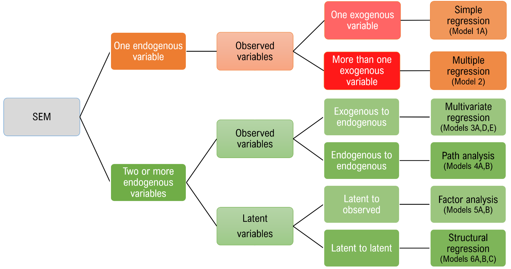
True or False. SEM encompasses a broad range of linear models and combines simultaneous linear equations with latent variable modeling.
Answer: True. Multivariate regression and path analysis are simultaneous equations of observed variables; factor analysis is a latent variable model, and structural regression combines the concepts of path analysis with factor analysis.
True or False. Multivariate regression means that there is always more than one exogenous predictor in my model.
Answer: False. Multivariate regression indicates more than one endogenous variable. You can certainly have only one exogenous predictor of multiple endogenous variables.
True or False. Structural regression models the regression paths only among latent variables.
Answer: True. Structural regression defines relationships between latent variables and path analysis defines relationships between observed variables.
References
Books
Jöreskog, K. G., Olsson, U. H., & Wallentin, F. Y. (2016). Multivariate analysis with LISREL. Basel, Switzerland: Springer.
Kline, R. B. (2016). Principles and practice of structural equation modeling (4th ed.). Guilford publications.
For more information on:
- lavaan’s own tutorial http://lavaan.ugent.be/tutorial
- extracting objects from lavaan Inspect or extract information from a fitted lavaan object
Saturated versus baseline models
Fit indexes