Survey Data Analysis with R
Why do we need survey data analysis software?
Regular procedures in statistical software (that is not designed for survey data) analyzes data as if the data were collected using simple random sampling. For experimental and quasi-experimental designs, this is exactly what we want. However, very few surveys use a simple random sample to collect data. Not only is it nearly impossible to do so, but it is not as efficient (either financially and statistically) as other sampling methods. When any sampling method other than simple random sampling is used, we usually need to use survey data analysis software to take into account the differences between the design that was used to collect the data and simple random sampling. This is because the sampling design affects both the calculation of the point estimates and the standard errors of those estimates. If you ignore the sampling design, e.g., if you assume simple random sampling when another type of sampling design was used, both the point estimates and their standard errors will likely be calculated incorrectly. The sampling weight will affect the calculation of the point estimate, and the stratification and/or clustering will affect the calculation of the standard errors. Ignoring the clustering will likely lead to standard errors that are underestimated, possibly leading to results that seem to be statistically significant, when in fact, they are not. The difference in point estimates and standard errors obtained using non-survey software and survey software with the design properly specified will vary from data set to data set, and even between analyses using the same data set. While it may be possible to get reasonably accurate results using non-survey software, there is no practical way to know beforehand how far off the results from non-survey software will be.
Sampling designs
Most people do not conduct their own surveys. Rather, they use survey data that some agency or company collected and made available to the public. The documentation must be read carefully to find out what kind of sampling design was used to collect the data. This is very important because many of the estimates and standard errors are calculated differently for the different sampling designs. Hence, if you mis-specify the sampling design, the point estimates and standard errors will likely be wrong.
Below are some common features of many sampling designs.
Sampling weights: There are several types of weights that can be associated with a survey. Perhaps the most common is the sampling weight. A sampling weight is a probability weight that has had one or more adjustments made to it. Both a sampling weight and a probability weight are used to weight the sample back to the population from which the sample was drawn. By definition, a probability weight is the inverse of the probability of being included in the sample due to the sampling design (except for a certainty PSU, see below). The probability weight is calculated as N/n, where N = the number of elements in the population and n = the number of elements in the sample. For example, if a population has 10 elements and 3 are sampled at random with replacement, then the probability weight would be 10/3 = 3.33. In a two-stage design, the probability weight is calculated as f1f2, which means that the inverse of the sampling fraction for the first stage is multiplied by the inverse of the sampling fraction for the second stage. Under many sampling plans, the sum of the probability weights will equal the population total.
While many textbooks will end their discussion of probability weights here, this definition does not fully describe the sampling weights that are included with actual survey data sets. Rather, the sampling weight, which is sometimes called a “final weight,” starts with the inverse of the sampling fraction, but then incorporates several other values, such as corrections for unit non-response, errors in the sampling frame (sometimes called non-coverage), calibration and trimming. Because these other values are included in the probability weight that is included with the data set, it is often inadvisable to modify the sampling weights, such as trying to standardize them for a particular variable, e.g., age.
Strata: Stratification is a method of breaking up the population into different groups, often by demographic variables such as gender, race or SES. Each element in the population must belong to one, and only one, strata. Once the strata have been defined, samples are taken from each stratum as if it were independent of all of the other strata. For example, if a sample is to be stratified on gender, men and women would be sampled independently of one another. This means that the probability weights for men will likely be different from the probability weights for the women. In most cases, you need to have two or more PSUs in each stratum. The purpose of stratification is to reduce the standard error of the estimates, and stratification works most effectively when the variance of the dependent variable is smaller within the strata than in the sample as a whole.
PSU: This is the primary sampling unit. This is the first unit that is sampled in the design. For example, school districts from California may be sampled and then schools within districts may be sampled. The school district would be the PSU. If states from the US were sampled, and then school districts from within each state, and then schools from within each district, then states would be the PSU. One does not need to use the same sampling method at all levels of sampling. For example, probability-proportional-to-size sampling may be used at level 1 (to select states), while cluster sampling is used at level 2 (to select school districts). In the case of a simple random sample, the PSUs and the elementary units are the same. In general, accounting for the clustering in the data (i.e., using the PSUs), will increase the standard errors of the point estimates. Conversely, ignoring the PSUs will tend to yield standard errors that are too small, leading to false positives when doing significance tests.
FPC: This is the finite population correction. This is used when the sampling fraction (the number of elements or respondents sampled relative to the population) becomes large. The FPC is used in the calculation of the standard error of the estimate. If the value of the FPC is close to 1, it will have little impact and can be safely ignored. In some survey data analysis programs, such as SUDAAN, this information will be needed if you specify that the data were collected without replacement (see below for a definition of “without replacement”). The formula for calculating the FPC is ((N-n)/(N-1))1/2, where N is the number of elements in the population and n is the number of elements in the sample. To see the impact of the FPC for samples of various proportions, suppose that you had a population of 10,000 elements.
Sample size (n) FPC
1 1.0000
10 .9995
100 .9950
500 .9747
1000 .9487
5000 .7071
9000 .3162
Replicate weights: Replicate weights are a series of weight variables that are used to correct the standard errors for the sampling plan. They serve the same function as the PSU and strata variables (which are used a Taylor series linearization) to correct the standard errors of the estimates for the sampling design. Many public use data sets are now being released with replicate weights instead of PSUs and strata in an effort to more securely protect the identity of the respondents. In theory, the same standard errors will be obtained using either the PSU and strata or the replicate weights. There are different ways of creating replicate weights; the method used is determined by the sampling plan. The most common are balanced repeated and jackknife replicate weights. You will need to read the documentation for the survey data set carefully to learn what type of replicate weight is included in the data set; specifying the wrong type of replicate weight will likely lead to incorrect standard errors. For more information on replicate weights, please see Stata Library: Replicate Weights. Several statistical packages, including Stata, SAS, R, Mplus, SUDAAN and WesVar, allow the use of replicate weights. Another good source of information on replicate weights is Applied Survey Data Analysis, Second Edition by Steven G. Heeringa, Brady T. West and Patricia A. Berglund (2017, CRC Press).
Consequences of not using the design elements
Sampling design elements include the sampling weights, post-stratification weights (if provided), PSUs, strata, and replicate weights. Rarely are all of these elements included in a single public-use data set. However, ignoring the design elements that are included can often lead to inaccurate point estimates and/or inaccurate standard errors.
Sampling with and without replacement
Most samples collected in the real world are collected “without replacement”. This means that once a respondent has been selected to be in the sample and has participated in the survey, that particular respondent cannot be selected again to be in the sample. Many of the calculations change depending on if a sample is collected with or without replacement. Hence, programs like SUDAAN request that you specify if a survey sampling design was implemented with our without replacement, and an FPC is used if sampling without replacement is used, even if the value of the FPC is very close to one.
Examples
For the examples in this workshop, we will use the data set from NHANES 2011-2012. The data set and documentation can be downloaded from the NHANES web site. The data files can be downloaded as SAS.xpt files. The R script used for the workshop is here.
Reading the documentation
The first step in analyzing any survey data set is to read the documentation. With many of the public use data sets, the documentation can be quite extensive and sometimes even intimidating. Instead of trying to read the documentation “cover to cover”, there are some parts you will want to focus on. First, read the Introduction. This is usually an “easy read” and will orient you to the survey. There is usually a section or chapter called something like “Sample Design and Analysis Guidelines”, “Variance Estimation”, etc. This is the part that tells you about the design elements included with the survey and how to use them. Some even give example code. If multiple sampling weights have been included in the data set, there will be some instruction about when to use which one. If there is a section or chapter on missing data or imputation, please read that. This will tell you how missing data were handled. You should also read any documentation regarding the specific variables that you intend to use. As we will see little later on, we will need to look at the documentation to get the value labels for the variables. This is especially important because some of the values are actually missing data codes, and you need to do something so that R doesn’t treat those as valid values (or you will get some very “interesting” means, totals, etc.).
Downloading and installing the packages
You should use the following install.packages commands only once. The commands should be left in your R script file but commented out (by placing a “#” symbol before each).
install.packages("haven")
install.packages("survey")
install.packages("jtools")
install.packages("remotes")
remotes::install_github("carlganz/svrepmisc")
After the packages are downloaded, they need to be loaded. This needs to be done at the beginning of each R session.
library("haven")
library("survey")
library("jtools")
library("remotes")
library("svrepmisc")
Reading the data into R
The data are distributed from the NHANES website as SAS.xpt files. You can use the “foreign” package to read the data into R. The command will look like this:
nhanes2012 <- read_dta("D:/data/Seminars/Applied Survey Data Analysis R/nhanes2012_reduced.dta")
The variables
We will use about a dozen different variables in the examples in this workshop. Below is a brief summary of them. Some of the variables have been recoded to be binary variables (values of 2 recoded to a value of 0). The count of missing observations includes values truly missing as well as refused and don’t know.
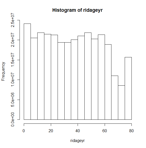
ridageyr – Age in years at exam – recoded; range of values: 0 – 79 are actual values, 80 = 80+ years of age
pad630 – How much time do you spend doing moderate-intensity activities on a type work day?; range of values: 10-960, 7053 missing observations
hsq496 – During the past 30 days, for about how many days have you felt worried, tense or anxious?; range of values: 0-30; 3073 missing observations
female – Recode of the variable riagendr; 0 = male, 1 = female; no missing observations
dmdborn4 – Country of birth; 1 = born in the United States, 0 = otherwise; 5 missing observations
dmdmartl – Marital status; 1 = married, 2 = widowed, 3 = divorced, 4 = separated, 5 = never married, 6 = living with partner; 4203 missing observations
dmdeduc2 – Education level of adults aged 20+ years; 1 = less than 9th grade, 2 = 9-11th grade, 3 = high school graduate, GED or equivalent, 4 = some college or AA degree, 5 = college graduate or above; 4201 missing observations
pad675 – How much time do you spend doing moderate-intensity sports, fitness, or recreation activities on a typical day?; range of values: 10-600; 6220 missing observations
hsq571 – During the past 12 months, have you donated blood?; 0 = no, 1 = yes; 3673 missing observations
pad680 – How much time do you usually spend sitting on a typical day?; range of values: 0-1380; 2365 missing observations
paq665 – Do you do any moderate-intensity sports, fitness or recreational activities that cause a small increase in breathing or heart rate at least 10 minutes continually?; 0 = no, 1 = yes; 2329 missing observations
hsd010 – Would you say that your general health is…; 1 = excellent, 2 = very good, 3 = good, 4 = fair, 5 = poor; 3064 missing observations
The svydesign function
Before we can start our analyses, we need to use the svydesign function from the “survey” package written by Thomas Lumley. The svydesign function tells R about the design elements in the survey. Once this command has been issued, all you need to do for your analyses is use the object that contains this information in each command. Because the 2011-2012 NHANES data were released with a sampling weight (wtint2yr), a PSU variable (sdmvpsu) and a strata variable (sdmvstra), we will use these our svydesign function. The svydesign function looks like this:
# nhanes2012 <- read_dta("D:/data/Seminars/Applied Survey Data Analysis R/nhanes2012_reduced.dta")
nhc <- svydesign(id=~sdmvpsu, weights=~wtint2yr,strata=~sdmvstra, nest=TRUE, survey.lonely.psu = "adjust", data=nhanes2012)
nhc
Stratified 1 - level Cluster Sampling design (with replacement)
With (31) clusters.
svydesign(id = ~sdmvpsu, weights = ~wtint2yr, strata = ~sdmvstra,
nest = TRUE, survey.lonely.psu = "adjust", data = nhanes2012)
We can get additional information about the sample, such as the number of PSUs per strata, by using the summary function.
summary(nhc)
Stratified 1 - level Cluster Sampling design (with replacement)
With (31) clusters.
svydesign(id = ~sdmvpsu, weights = ~wtint2yr, strata = ~sdmvstra,
    nest = TRUE, survey.lonely.psu = "adjust", data = nhanes2012)
Probabilities:
     Min.   1st Qu.    Median      Mean   3rd Qu.      Max.
4.541e-06 2.866e-05 5.526e-05 6.372e-05 8.809e-05 3.011e-04
Stratum Sizes:
            90  91  92  93  94  95  96  97  98  99 100 101 102 103
obs        862 998 875 602 688 722 676 608 708 682 700 715 624 296
design.PSU   3   3   3   2   2   2   2   2   2   2   2   2   2   2
actual.PSU   3   3   3   2   2   2   2   2   2   2   2   2   2   2
Data variables:
 [1] "dmdborn4" "dmdeduc2" "dmdmartl" "dmdyrsus" "female"   "hsd010"   "hsq496"
 [8] "hsq571"   "pad615"   "pad630"   "pad660"   "pad675"   "pad680"   "paq610"
[15] "paq625"   "paq640"   "paq655"   "paq665"   "paq670"   "paq710"   "paq715"
[22] "ridageyr" "sdmvpsu"  "sdmvstra" "seqn"     "wtint2yr"
Descriptive statistics with continuous variables
We will start with something simple: calculating the mean of a continuous variable. In this example, we use the variable ridageyr, which is the age of the respondent. Please note that the documentation for the svymean function, as well as other functions that provide descriptive statistics, is found in the section of the documentation called surveysummary.
svymean(~ridageyr, nhc)
           mean     SE
ridageyr   37.185   0.6965
We can also get the standard deviation of the age variable. We use the function svysd, which is found in the jtools package.
svysd(~ridageyr,design = nhc, na = TRUE)
            std. dev.
ridageyr    22.37
When there are missing data for a variable, the na = TRUE argument is needed.
svymean(~pad630, nhc, na = TRUE)
         mean     SE
pad630   139.89   5.5791
Here is another example.
svymean(~hsq496, nhc, na = TRUE)
         mean     SE
hsq496   5.3839   0.19
The means of more than one variable can be obtained by placing “+” between the variables. Notice that a listwise deletion has been done, so that the means in output below are different from the means shown above.
svymean(~ridageyr+pad630+hsq496, nhc, na = TRUE)
            mean      SE
ridageyr    41.9779   0.8212
pad630      139.7228  5.7137
hsq496      5.3739    0.2781
In the examples below, the mean, standard deviation, and variance are obtained.
svymean(~pad680, nhc, na = TRUE)
          mean     SE
pad680    391.3    5.986
svysd(~pad680,design = nhc, na = TRUE)
         std. dev.
pad680   200.846
svyvar(~pad680, design = nhc, na = TRUE)
          variance     SE
pad680    40339        827.77
The cv function is used to get the coefficient of variation. The coefficient of variation is the ratio of the standard error to the mean, multiplied by 100%. It is an indication of the variability relative to the mean in the population and is not affected by the unit of measurement of the variable.
cv(svymean(~pad680,design = nhc, na = TRUE))
pad680
pad680   0.01529783
Below is an example of how to obtain the design effect (Deff). The Deff is a ratio of two variances. In the numerator we have the variance estimate from the current sample (including all of its design elements), and in the denominator we have the variance from a hypothetical sample of the same size drawn as an SRS. In other words, the Deff tells you how efficient your sample is compared to an SRS of equal size. If the Deff is less than 1, your sample is more efficient than SRS; usually the Deff is greater than 1. In the example below, the Deff is 5.9887. This means that a sample drawn using the current sampling plan needs to be six times the size needed if the sample was collected via an SRS. The Deff is specific to a variable, so some variables may have larger or smaller Deffs.
svymean(~pad680, nhc, na = TRUE, deff = TRUE)
          mean      SE       DEff
pad680    391.300   5.986    5.9887
Quantiles are a useful descriptive statistic for continuous variables, particularly variables that are not normally distributed.
svyquantile(~hsq496, design = nhc, na = TRUE, c(.25,.5,.75),ci=TRUE)
$quantiles
         0.25   0.5   0.75
hsq496   0      1     5

$CIs
, , hsq496

          0.25   0.5   0.75
(lower    0      1     5
upper)    0      2     7
Let’s get some descriptive statistics for binary variables. We have some choices here. Let’s start by getting the mean of the variable female, which is coded 1 for females and 0 for males. Taking the mean of a variable that is coded 0/1 gives the proportion of 1s, so the mean of this variable is the estimated proportion of the population that is female.
# means and proportions for binary variables
svymean(~female, nhc)
           mean      SE
female     0.51195   0.0064
We can use the confint function to get the confidence interval around this mean.
confint(svymean(~female, nhc))
         2.5 %       97.5 %
female   0.4993307   0.5245742
However, comment on page 70of the documentation for the survey package, we should use svyciprop rather than confint. There are several options that can be supplied for the method argument. Please see pages 70-71 of the documentation. The likelihood option uses the (Rao-Scott) scaled chi-squared distribution for the log likelihood from a binomial distribution.
svyciprop(~I(female==1), nhc, method="likelihood")
               2.5%    97.5%
I(female == 1) 0.512   0.498 0.53
# li is short for likelihood
svyciprop(~I(female==0), nhc, method="li")
               2.5%    97.5%
I(female == 0) 0.488   0.474 0.5
The logit option fits a logistic regression model and computes a Wald-type interval on the log-odds scale, which is then transformed to the probability scale.
svyciprop(~I(female==1), nhc, method="logit")
               2.5%     97.5%
I(female == 1) 0.512    0.498 0.53
The xlogit option uses a logit transformation of the mean and then back-transforms to the probability scale. This appears to be the method used by SUDAAN and SPSS COMPLEX SAMPLES.
 svyciprop(~I(female==1), nhc, method="xlogit")
               2.5%    97.5%
I(female == 1) 0.512   0.498 0.53
As stated on page 71 of the documentation, the use of the mean option (shortened in the code below to me), reproduces the results given by Stata’s svy: mean command.
svyciprop(~I(female==1), nhc, method="me", df=degf(nhc))
               2.5%    97.5%
I(female == 1) 0.512   0.498 0.53
As stated on page 71 of the documentation, the use of the mean option (shortened in the code below to me), reproduces the results given by Stata’s svy: prop command.
svyciprop(~I(female==1), nhc, method="lo", df=degf(nhc))
               2.5%     97.5%
I(female == 1) 0.512    0.498 0.53
You can also get the proportions of 0s, as shown below.
svyciprop(~I(female==0), nhc, method="mean")
               2.5%    97.5%
I(female == 0) 0.488   0.474 0.5
Below is another way to get the proportions of 1s. The point of these examples is that you can use this type of syntax to get the proportion of any level of a categorical variable.
svyciprop(~I(female==1), nhc, method="mean")
               2.5%    97.5%
I(female == 1) 0.512   0.498 0.53
Finally, let’s see how to get totals. We will use the svytotal function.
svytotal(~dmdborn4,design = nhc, na = TRUE)
             total       SE
dmdborn4     260493506   19670647
In the next example, we will get the coefficient of variation for this total.
cv(svytotal(~dmdborn4,design = nhc, na = TRUE))
         dmdborn4
dmdborn4 0.075513
Let’s get the design effect for the total.
svytotal(~dmdborn4,design = nhc, na = TRUE, deff = TRUE)
             total        SE          DEff
dmdborn4     260493506    19670647   314.9
Descriptive statistics for categorical variables
Let’s see some ways to get descriptive statistics for categorical variables, whether or not these variables are binary. We will start with the table function. In the example below, we get the frequencies for the variable female.
svytable(~female, design = nhc)
female
0           1
149630839   156959842
We can also use the table function to get crosstabulations. We will start with two-way crosstabs.
# 2-way
svytable(~female+dmdborn4, nhc)
dmdborn4
female   0         1
0       22449131   127102676
1       23543299   133390830
In the next example, we use a different syntax to do the same thing. Notice that the output is displayed differently, although the information in the output is the same.
# 2-way
svytable(~interaction(female, dmdborn4), design = nhc)
interaction(female, dmdborn4)
0.0        1.0        0.1         1.1
22449131   23543299   127102676   133390830
Now let’s get a three-way table.
# 3-way
svytable(~interaction(female, dmdborn4, hsq571), design = nhc)
interaction(female, dmdborn4, hsq571)
0.0.0        1.0.0        0.1.0        1.1.0        0.0.1      1.0.1      0.1.1       1.1.1
16994772.6   16101456.8   78140097.2   83984812.9   503957.9   277883.3   7083759.3   6155573.1
Let’s go a little crazy and get a four-way table.
# 4-way
svytable(~interaction(female, dmdborn4, hsq571, paq665), design = nhc)
interaction(female, dmdborn4, hsq571, paq665)
0.0.0.0     1.0.0.0     0.1.0.0     1.1.0.0     0.0.1.0     1.0.1.0     0.1.1.0
9742281.10  9259759.05  41213690.37 43983640.78 314995.28   95874.61    2938039.53
1.1.1.0     0.0.0.1     1.0.0.1     0.1.0.1     1.1.0.1     0.0.1.1     1.0.1.1
2587794.24  7252491.54  6841697.75  36908800.64 40001172.12 188962.61   182008.74
0.1.1.1     1.1.1.1
4145719.79  3567778.91
Although not a descriptive statistic, let’s see how to get a chi-squared test while we are talking about tables. Of course, only a two-way table can be specified.
svychisq(~female+dmdborn4, nhc, statistic="adjWald")

Design-based Wald test of association

data: svychisq(~female + dmdborn4, nhc, statistic = "adjWald")
F = 0.00019185, ndf = 1, ddf = 17, p-value = 0.9891
Graphing of continuous variables
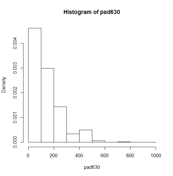
Let’s start with a histogram. By default, the density is shown on the y-axis.
svyhist(~pad630, nhc)
Instead of the density on the y-axis, we can request the count. Notice the large count of respondents in the last column on the right. The coding of the ridageyr variable explains this.
svyhist(~ridageyr, nhc, probability = FALSE)
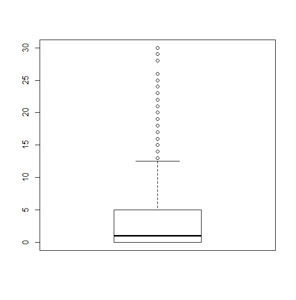
We can also create boxplots.
svyboxplot(~hsq496~1, nhc, all.outliers=TRUE)
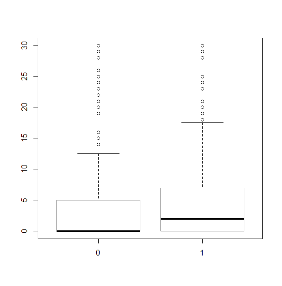
We can break the boxplot by a grouping variable. The grouping variable must be a factor.
svyboxplot(~hsq496~factor(female), nhc, all.outliers=TRUE)
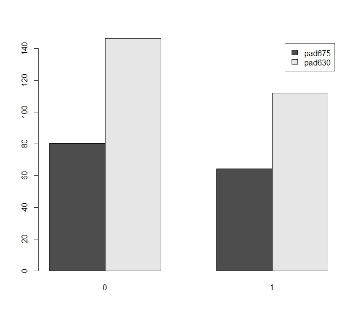
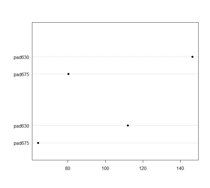
We can make barcharts. In the example below, we also preview some syntax used for subpopulation analysis.
barplt<-svyby(~pad675+pad630, ~female, nhc, na = TRUE, svymean)
barplot(barplt,beside=TRUE,legend=TRUE)
dotchart(barplt)
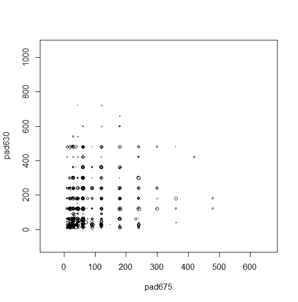
We can make a scatterplot with the sampling weights corresponding to the bubble size.
svyplot(~pad675+pad630, nhc, style="bubble")
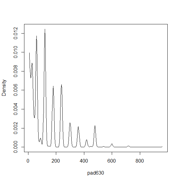
There are a variety of density and smoothed plots that can be made. Some examples are below.
smth<-svysmooth(~pad630, design=nhc)
plot(smth)
dens<-svysmooth(~pad630, design=nhc,bandwidth=30)
plot(dens)
dens1<-svysmooth(~pad630, design=nhc)
plot(dens1)
Subpopulation Analysis
Before we continue with our descriptive statistics, we should pause to discuss the analysis of subpopulations. The analysis of subpopulations is one place where survey data and experimental data are quite different. If you have data from an experiment (or quasi-experiment), and you want to analyze the responses from, say, just the women, or just people over age 50, you can just delete the unwanted cases from the data set or use the by: prefix. Complex survey data are different. With survey data, you (almost) never get to delete any cases from the data set, even if you will never use them in any of your analyses. Instead, the survey package has two options that allow you to correctly analyze subpopulations of your survey data. These options are svyby and subset.survey.design. The subset.survey.design option is sort of like deleting unwanted cases (without really deleting them, of course), and the svyby option is very similar to by-group processing in that the results are shown for each group of the by-variable.
First, however, let’s take a second to see why deleting cases from a survey data set can be so problematic. There are two formulas that can used to calculate the standard errors. One formula is used when you do by-group processing or delete unwanted cases from the dataset, and survey statisticians call this the conditional approach. This is used when members of the subpopulation cannot appear in certain strata and therefore those strata should not be used in the calculation of the standard error. In practice, this rarely happens in public-use complex survey datasets. One reason is because the analyst usually does not know which combination of variables defines a particular stratum.
The other formula is used when you use the svyby option, and survey statisticians call this the unconditional approach. This is used when members of the subpopulation can be in any of the strata, even if there are some strata in the sample data that do not contain any members of the subpopulation. Because members of the subpopulation, all of the strata need to be used in the calculation of the standard error, and hence all of the data must be in the dataset. If the data set is subset (meaning that observations not to be included in the subpopulation are deleted from the data set), the standard errors of the estimates cannot be calculated correctly. When the svyby option is used, only the cases defined by the subpopulation are used in the calculation of the estimate, but all cases are used in the calculation of the standard errors. For more information on this issue, please see Sampling Techniques, Third Edition by William G. Cochran (1977) and Small Area Estimation by J. N. K. Rao (2003). A nice description of this issue given in Brady West’s 2009 Stata Conference (in Washington, D.C.).
Both svyby and subset.svy.design use the formula for the unconditional standard errors.
Let’s start by calculating the mean of age.
svymean(~ridageyr, nhc)
           mean     SE
ridageyr   37.185   0.6965
Now let’s calculate the mean of age for males and females. In this example, the variable female is the subpopulation variable.
svyby(~ridageyr, ~female, nhc, svymean)
female   ridageyr   se
0 0      36.22918   0.8431945
1 1      38.09657   0.6713502
You can use more than one categorical variable to define the subpopulation. To do so, put + between the variables.
svyby(~ridageyr, ~dmdmartl+female, nhc, svymean)
      dmdmartl female   ridageyr   se
1.0   1        0        51.34608   0.7473752
2.0   2        0        67.49342   2.6062013
3.0   3        0        52.42614   0.7270806
4.0   4        0        47.16402   1.2085674
5.0   5        0        33.78962   1.3163405
6.0   6        0        40.55277   1.8945413
1.1   1        1        49.33443   0.6176356
2.1   2        1        71.39812   0.8627829
3.1   3        1        53.22067   0.7138037
4.1   4        1        47.16444   1.2200152
5.1   5        1        33.64747   1.4922117
6.1   6        1        35.94412   1.4423662
In the next example, three variables are used.
svyby(~pad630, ~dmdmartl+dmdeduc2+female, nhc, na = TRUE, svymean)
        dmdmartl   dmdeduc2   female  pad630      se
1.1.0   1          1          0       175.26250   28.12358
2.1.0   2          1          0       187.34360   62.96688
3.1.0   3          1          0       0.00000     0.00000
4.1.0   4          1          0       205.13325   35.53482
5.1.0   5          1          0       221.33212   60.76421
6.1.0   6          1          0       188.91514   71.24062
1.2.0   1          2          0       191.89233   18.18910
2.2.0   2          2          0       167.20401   14.10054
3.2.0   3          2          0       238.10555   29.71073
4.2.0   4          2          0       199.08510   38.03347
5.2.0   5          2          0       260.45360   41.06904
6.2.0   6          2          0       257.39812   43.61217
1.3.0   1          3          0       165.88490   9.75834
2.3.0   2          3          0       103.25693   20.07422
3.3.0   3          3          0       159.62009   17.52999
4.3.0   4          3          0       279.83812   48.20102
5.3.0   5          3          0       169.78003   18.53166
6.3.0   6          3          0       215.15772   24.03397
1.4.0   1          4          0       155.18399   13.21638
2.4.0   2          4          0       125.93947   35.75450
3.4.0   3          4          0       271.14720   56.91977
4.4.0   4          4          0       81.12185    29.50234
5.4.0   5          4          0       125.94122   11.38165
6.4.0   6          4          0       198.18129   25.91694
1.5.0   1          5          0       133.26699   10.84879
2.5.0   2          5          0       123.88774   52.93405
3.5.0   3          5          0       181.38341   33.00260
4.5.0   4          5          0       237.32606   84.81068
5.5.0   5          5          0       104.57660   26.15903
6.5.0   6          5          0       105.54748   7.58048
1.1.1   1          1          1       123.18726   33.99413
2.1.1   2          1          1       176.09593   72.50964
3.1.1   3          1          1        54.28887   15.49709
4.1.1   4          1          1       169.35988   80.57609
5.1.1   5          1          1       309.99124   93.15230
6.1.1   6          1          1       120.00000    0.00000
1.2.1   1          2          1       143.36162   14.00536
2.2.1   2          2          1        90.60535   17.21293
3.2.1   3          2          1       163.20222   47.28731
4.2.1   4          2          1       165.84824   46.57393
5.2.1   5          2          1       166.33346   46.45898
6.2.1   6          2          1       144.99504   24.39718
1.3.1   1          3          1       111.80803   12.92772
2.3.1   2          3          1       110.48051   37.21189
3.3.1   3          3          1       145.50738   25.43471
4.3.1   4          3          1       302.02249   117.29823
5.3.1   5          3          1       190.28528   55.64751
6.3.1   6          3          1        98.81543   21.16077
1.4.1   1          4          1       146.28879   22.89246
2.4.1   2          4          1       101.83852   11.74256
3.4.1   3          4          1       129.58833   28.49053
4.4.1   4          4          1       142.53219   26.01105
5.4.1   5          4          1       109.54923   15.62974
6.4.1   6          4          1       152.59225   23.74680
1.5.1   1          5          1        88.91933    8.30694
2.5.1   2          5          1       260.99621   63.18704
3.5.1   3          5          1        76.00663   11.32266
4.5.1   4          5          1       117.92163   34.79595
5.5.1   5          5          1       126.51918   19.29269
6.5.1   6          5          1        89.01130   23.17592
Sometimes you don’t want so much output. Rather, you just want the output for a specific group. You can get this by creating a subpopulation of the data with the subset function. In the example below, we obtain the output only for males.
smale <- subset(nhc,female == 0)
summary(smale)
Stratified 1 - level Cluster Sampling design (with replacement)
With (31) clusters.
subset(nhc, female == 0)
Probabilities:
Min. 1st Qu. Median Mean 3rd Qu. Max.
5.095e-06 3.044e-05 5.680e-05 6.521e-05 9.250e-05 2.326e-04
Stratum Sizes:
90 91 92 93 94 95 96 97 98 99 100 101 102 103
obs 426 496 452 288 351 355 353 289 352 338 355 357 315 129
design.PSU 3 3 3 2 2 2 2 2 2 2 2 2 2 2
actual.PSU 3 3 3 2 2 2 2 2 2 2 2 2 2 2
Data variables:
[1] "dmdborn4" "dmdeduc2" "dmdmartl" "dmdyrsus" "female" "hsd010" "hsq496"
[8] "hsq571" "pad615" "pad630" "pad660" "pad675" "pad680" "paq610"
[15] "paq625" "paq640" "paq655" "paq665" "paq670" "paq710" "paq715"
[22] "ridageyr" "sdmvpsu" "sdmvstra" "seqn" "wtint2yr"
svymean(~ridageyr,design=smale)
           mean     SE
ridageyr   36.229   0.8432
Models
A wide variety of statistical models can be run with complex survey data. With only a few exceptions, the results of these analyses can be interpreted just as the results from the same analyses with experimental or quasi-experimental data. For example, if you run an OLS regression with weighted data, assuming that the sampling plan has been correctly specified, the regression coefficients are interpreted exactly as any other OLS regression coefficient. The same is true for the various logistic regression models, including binary logistic regression, ordinal logistic regression and multinomial logistic regression (of which there is not an example in this workshop). Most of the assumptions of these models are also the same. However, some assumptions, such as the assumption regarding the normality of the residuals in OLS regression, are often not meaningful because of the large sample size commonly seen with complex survey data.
t-tests
Let’s start doing some simple statistics. One-sample, paired-sample and independent-samples t-tests can be run with the svyttest function.
A one-sample t-test is shown below.
svyttest(pad675~0, nhc, na = TRUE)

	Design-based one-sample t-test

data:  pad675 ~ 0
t = 40.447, df = 16, p-value < 2.2e-16
alternative hypothesis: true mean is not equal to 0
95 percent confidence interval:
 63.84046 70.90254
sample estimates:
   mean
67.3715
In the example of the paired-samples t-test below, the “I” is used to tell R to leave the part in parentheses “as is”, meaning do the subtraction between the two variables. Hence, the formula means that the difference between
svyttest(I(pad660-pad675)~0, nhc, na = TRUE)

Design-based one-sample t-test

data: I(pad660 - pad675) ~ 0
t = 3.3059, df = 16, p-value = 0.004464
alternative hypothesis: true mean is not equal to 0
95 percent confidence interval:
2.718683 12.437915
sample estimates:
mean
7.578299
Now let’s run an independent-samples t-test.
svyttest(pad630~female, nhc)

Design-based t-test

data: pad630 ~ female
t = -5.6277, df = 16, p-value = 3.779e-05
alternative hypothesis: true difference in mean is not equal to 0
95 percent confidence interval:
-45.76433 -22.12149
sample estimates:
difference in mean
-33.94291
As you probably know, an independent-samples t-test tests the null hypothesis that the difference in the means of the two groups is 0. Another way to think about this type of t-test is to think of it as a linear regression with a single binary predictor. The intercept will be the mean of the reference group, and the coefficient will be the difference between the two groups.
We will start by running the t-test function as before, and then replicate the results using the svyglm function, which can be used to run a linear regression. The svyby function is used with the covmat argument to save the elements to a matrix so that we can use the svycontrast function to subtract the values. The purpose of this example is not to belabor the point about a t-test, but rather to show how to get a matrix of values and then compare those values with the svycontrast function in a simple example where the answer is already known.
svyttest(ridageyr~female, nhc)

Design-based t-test

data: ridageyr ~ female
t = 2.9691, df = 16, p-value = 0.009043
alternative hypothesis: true difference in mean is not equal to 0
95 percent confidence interval:
0.634692 3.100076
sample estimates:
difference in mean
1.867384
summary(svyglm(ridageyr~female, design=nhc))

Call:
svyglm(formula = ridageyr ~ female, design = nhc)

Survey design:
svydesign(id = ~sdmvpsu, weights = ~wtint2yr, strata = ~sdmvstra,
nest = TRUE, survey.lonely.psu = "adjust", data = nhanes2012)

Coefficients:
Estimate Std. Error t value Pr(>|t|)
(Intercept) 36.2292 0.8432 42.967 < 2e-16 ***
female 1.8674 0.6289 2.969 0.00904 **
---
Signif. codes: 0 ‘***’ 0.001 ‘**’ 0.01 ‘*’ 0.05 ‘.’ 0.1 ‘ ’ 1

(Dispersion parameter for gaussian family taken to be 499.5325)

Number of Fisher Scoring iterations: 2
a <- svyby(~ridageyr, ~female, nhc, na.rm.by = TRUE, svymean, covmat = TRUE)
vcov(a)
0           1
0 0.7109769 0.3830638
1 0.3830638 0.4507111
a
female  ridageyr   se
0 0     36.22918   0.8431945
1 1     38.09657   0.6713502
svycontrast(a, c( -1, 1))
          contrast   SE
contrast  1.8674     0.6289
        # 4.589723 - 6.153479
This example is similar to the previous example, except that here the svypredmeans function is used.
summary(svyglm(pad630~female, design=nhc))

Call:
svyglm(formula = pad630 ~ female, design = nhc)

Survey design:
svydesign(id = ~sdmvpsu, weights = ~wtint2yr, strata = ~sdmvstra,
nest = TRUE, survey.lonely.psu = "adjust", data = nhanes2012)

Coefficients:
            Estimate   Std. Error   t value   Pr(>|t|)
(Intercept) 155.627    7.008        22.206    1.90e-13 ***
female      -33.943    6.031        -5.628    3.78e-05 ***
---
Signif. codes: 0 ‘***’ 0.001 ‘**’ 0.01 ‘*’ 0.05 ‘.’ 0.1 ‘ ’ 1

(Dispersion parameter for gaussian family taken to be 21951.7)

Number of Fisher Scoring iterations: 2
Note that the variable female cannot be in model if you want to get the predicted means for that variable.
ttest1 <- (svyglm(ridageyr~1, design=nhc))
summary(ttest1)

Call:
svyglm(formula = ridageyr ~ 1, design = nhc)

Survey design:
svydesign(id = ~sdmvpsu, weights = ~wtint2yr, strata = ~sdmvstra,
nest = TRUE, survey.lonely.psu = "adjust", data = nhanes2012)

Coefficients:
            Estimate   Std. Error   t value   Pr(>|t|)
(Intercept) 37.1852    0.6965       53.39     <2e-16 ***
---
Signif. codes: 0 ‘***’ 0.001 ‘**’ 0.01 ‘*’ 0.05 ‘.’ 0.1 ‘ ’ 1

(Dispersion parameter for gaussian family taken to be 500.4039)

Number of Fisher Scoring iterations: 2
The variable female is used here to get the predicted means for each level of female.
svypredmeans(ttest1, ~female)
   mean    SE
0  36.229  0.8432
1  38.097  0.6714
tt<-svyttest(pad630~female, nhc)
tt

Design-based t-test

data: pad630 ~ female
t = -5.6277, df = 16, p-value = 3.779e-05
alternative hypothesis: true difference in mean is not equal to 0
95 percent confidence interval:
-45.76433 -22.12149
sample estimates:
difference in mean
-33.94291
We can get the confidence interval around the difference. In this example, we get the 90% confidence interval.
confint(tt, level=0.9)
[1] -43.67864 -24.20718
attr(,"conf.level")
[1] 0.9
Multiple linear regression
We need to use the summary function to get the standard errors, test statistics and p-values. Let’s start with a model that has no interaction terms. The outcome variable will be pad630, and the predictors will be female and hsq571.
summary(svyglm(pad630~female+hsq571, design=nhc, na.action = na.omit))

Call:
svyglm(formula = pad630 ~ female + hsq571, design = nhc, na.action = na.omit)

Survey design:
svydesign(id = ~sdmvpsu, weights = ~wtint2yr, strata = ~sdmvstra,
nest = TRUE, survey.lonely.psu = "adjust", data = nhanes2012)

Coefficients:
            Estimate   Std. Error t value   Pr(>|t|)
(Intercept) 164.707    6.595      24.975    1.24e-13 ***
female      -39.296    6.325      -6.212    1.66e-05 ***
hsq571      -11.722    20.267     -0.578    0.572
---
Signif. codes: 0 ‘***’ 0.001 ‘**’ 0.01 ‘*’ 0.05 ‘.’ 0.1 ‘ ’ 1

(Dispersion parameter for gaussian family taken to be 23558.77)

Number of Fisher Scoring iterations: 2
Now let’s add an interaction between the two predictor variables.
summary(svyglm(pad630~female*hsq571, design=nhc, na.action = na.omit))

Call:
svyglm(formula = pad630 ~ female * hsq571, design = nhc, na.action = na.omit)

Survey design:
svydesign(id = ~sdmvpsu, weights = ~wtint2yr, strata = ~sdmvstra,
nest = TRUE, survey.lonely.psu = "adjust", data = nhanes2012)

Coefficients:
               Estimate   Std. Error  t value   Pr(>|t|)
(Intercept)     167.107   6.847       24.404    7.13e-13 ***
female          -44.520   6.827       -6.521    1.35e-05 ***
hsq571          -40.975   18.282      -2.241    0.04174 *
female:hsq571   67.630    19.484       3.471    0.00374 **
---
Signif. codes: 0 ‘***’ 0.001 ‘**’ 0.01 ‘*’ 0.05 ‘.’ 0.1 ‘ ’ 1

(Dispersion parameter for gaussian family taken to be 23441.51)

Number of Fisher Scoring iterations: 2
glm1 <- (svyglm(pad630~female*hsq571, design=nhc, na.action = na.omit))
glm1
Stratified 1 - level Cluster Sampling design (with replacement)
With (31) clusters.
svydesign(id = ~sdmvpsu, weights = ~wtint2yr, strata = ~sdmvstra,
nest = TRUE, survey.lonely.psu = "adjust", data = nhanes2012)

Call: svyglm(formula = pad630 ~ female * hsq571, design = nhc, na.action = na.omit)

Coefficients:
(Intercept)   female   hsq571   female:hsq571
 167.11      -44.52    -40.97   67.63

Degrees of Freedom: 1672 Total (i.e. Null); 14 Residual
(8083 observations deleted due to missingness)
Null Deviance: 40340000
Residual Deviance: 39190000 AIC: 21580
confint(glm1)
                2.5 %       97.5 %
(Intercept)     153.68606   180.527513
female          -57.89966   -31.139511
hsq571          -76.80715   -5.141942
female:hsq571    29.44252   105.817225
This example is just like the previous one, only here factor notation is used. This is important when the categorical predictor has more than two levels.
summary(svyglm(pad630~factor(female)*factor(dmdmartl), design=nhc, na.action = na.omit))

Call:
svyglm(formula = pad630 ~ factor(female) * factor(dmdmartl),
    design = nhc, na.action = na.omit)

Survey design:
svydesign(id = ~sdmvpsu, weights = ~wtint2yr, strata = ~sdmvstra,
    nest = TRUE, survey.lonely.psu = "adjust", data = nhanes2012)

Coefficients:
                                    Estimate    Std. Error   t value   Pr(>|t|)
(Intercept)                         156.694      8.766        17.876    1.97e-06 ***
factor(female)1                     -38.069      12.438       -3.061    0.0222 *
factor(dmdmartl)2                   -24.083      23.185       -1.039    0.3390
factor(dmdmartl)3                    52.729      28.804        1.831    0.1169
factor(dmdmartl)4                    31.274      32.355        0.967    0.3711
factor(dmdmartl)5                   -10.271      13.330       -0.771    0.4702
factor(dmdmartl)6                    44.728      16.959        2.637    0.0387 *
factor(female)1:factor(dmdmartl)2    26.414      28.913        0.914    0.3962
factor(female)1:factor(dmdmartl)3   -46.720      43.539       -1.073    0.3245
factor(female)1:factor(dmdmartl)4    51.033      51.334        0.994    0.3585
factor(female)1:factor(dmdmartl)5    23.355      18.086        1.291    0.2441
factor(female)1:factor(dmdmartl)6   -40.780      25.360       -1.608    0.1589
---
Signif. codes:  0 ‘***’ 0.001 ‘**’ 0.01 ‘*’ 0.05 ‘.’ 0.1 ‘ ’ 1

(Dispersion parameter for gaussian family taken to be 23215.65)

Number of Fisher Scoring iterations: 2

ols1 <- (svyglm(pad630~1, design=nhc, na.action = na.omit))
predmarg<-svypredmeans(ols1, ~interaction(female,dmdmartl))
predmarg
      mean      SE
1.1   118.63    9.5904
0.6   201.42   13.4189
0.1   156.69    8.7656
0.5   146.42   12.3533
1.5   131.71   13.3056
1.4   200.93   52.4999
1.6   122.57   14.8851
0.3   209.42   27.2862
1.2   120.96   11.1044
1.3   124.63   15.5059
0.4   187.97   38.8611
0.2   132.61   20.7758
Non-parametric tests
Non-parametric tests can also be done. Let’s start with a Wilcoxon signed rank test, which is the non-parametric analog of an independent-samples t-test.
wil <- svyranktest(hsq496~female, design = nhc, na = TRUE, test = c("wilcoxon"))
wil

Design-based KruskalWallis test

data: hsq496 ~ female
t = 6.3291, df = 16, p-value = 1.002e-05
alternative hypothesis: true difference in mean rank score is not equal to 0
sample estimates:
difference in mean rank score
0.06896535
This is an example of a median test.
mtest <- svyranktest(hsq496~female, design = nhc, na = TRUE, test=("median"))
mtest

Design-based median test

data: hsq496 ~ female
t = 4.9504, df = 16, p-value = 0.0001446
alternative hypothesis: true difference in mean rank score is not equal to 0
sample estimates:
difference in mean rank score
0.11726
This is an example of a Kruskal Wallis test, which is the non-parametric analog of a one-way ANOVA.
kwtest <- svyranktest(hsq496~female, design = nhc, na = TRUE, test=("KruskalWallis"))
kwtest

Design-based KruskalWallis test

data: hsq496 ~ female
t = 6.3291, df = 16, p-value = 1.002e-05
alternative hypothesis: true difference in mean rank score is not equal to 0
sample estimates:
difference in mean rank score
0.06896535
Logistic regression
Let’s see a few examples of logistic regression.
logit1 <- (svyglm(paq665~factor(hsd010)+ridageyr, family=quasibinomial, design=nhc, na.action = na.omit))
summary(logit1)

Call:
svyglm(formula = paq665 ~ factor(hsd010) + ridageyr, design = nhc,
family = quasibinomial, na.action = na.omit)

Survey design:
svydesign(id = ~sdmvpsu, weights = ~wtint2yr, strata = ~sdmvstra,
nest = TRUE, survey.lonely.psu = "adjust", data = nhanes2012)

Coefficients:
Estimate Std. Error t value Pr(>|t|)
(Intercept) 0.717830 0.123638 5.806 8.40e-05 ***
factor(hsd010)2 -0.053653 0.099863 -0.537 0.600902
factor(hsd010)3 -0.541820 0.104759 -5.172 0.000232 ***
factor(hsd010)4 -0.981956 0.103744 -9.465 6.46e-07 ***
factor(hsd010)5 -1.882124 0.201158 -9.356 7.31e-07 ***
ridageyr -0.009443 0.002191 -4.311 0.001013 **
---
Signif. codes: 0 ‘***’ 0.001 ‘**’ 0.01 ‘*’ 0.05 ‘.’ 0.1 ‘ ’ 1

(Dispersion parameter for quasibinomial family taken to be 1.219511)

Number of Fisher Scoring iterations: 4
In the next example, we will run the logistic regression on a subpopulation (respondents over age 20).
subset1 <- subset(nhc, ridageyr > 20)
logit2 <- (svyglm(paq665~factor(hsd010)+ridageyr, family=quasibinomial, design=subset1, na.action = na.omit))
summary(logit2)

Call:
svyglm(formula = paq665 ~ factor(hsd010) + ridageyr, design = subset1,
family = quasibinomial, na.action = na.omit)

Survey design:
subset(nhc, ridageyr > 20)

Coefficients:
                   Estimate   Std. Error    t value    Pr(>|t|)
(Intercept)        0.86401    0.17432       4.956      0.000333 ***
factor(hsd010)2   -0.10723    0.11507      -0.932      0.369739
factor(hsd010)3   -0.59868    0.11209      -5.341      0.000176 ***
factor(hsd010)4   -1.09325    0.11226      -9.738      4.77e-07 ***
factor(hsd010)5   -2.04923    0.19386      -10.571     1.96e-07 ***
ridageyr          -0.01097    0.00292      -3.756      0.002740 **
---
Signif. codes: 0 ‘***’ 0.001 ‘**’ 0.01 ‘*’ 0.05 ‘.’ 0.1 ‘ ’ 1

(Dispersion parameter for quasibinomial family taken to be 1.024088)

Number of Fisher Scoring iterations: 4
We can also get a Wald test for a variable in the model.
regTermTest(logit2, ~ridageyr)
Wald test for ridageyr
in svyglm(formula = paq665 ~ factor(hsd010) + ridageyr, design = subset1,
family = quasibinomial, na.action = na.omit)
F = 14.10816 on 1 and 12 df: p= 0.0027404
Instead of getting an R-squared value as you do in linear regression, a pseudo-R-squared is given in logistic regression. There are many different versions of pseudo-R-squared, and two of them are available with the psrsq function.
psrsq(logit2, method = c("Cox-Snell"))
[1] 0.05148869
psrsq(logit2, method = c("Nagelkerke"))
[1] 0.06873682
Ordered logistic regression
Below is an example of an ordered logistic regression. Note that the outcome variable must be a factor.
ologit1 <- svyolr(factor(dmdeduc2)~factor(female)+factor(dmdborn4)+pad680, design = nhc, method = c("logistic"))
summary(ologit1)
Call:
svyolr(factor(dmdeduc2) ~ factor(female) + factor(dmdborn4) +
pad680, design = nhc, method = c("logistic"))

Coefficients:
                    Value          Std. Error       t value
factor(female)1     0.097569476    0.0487417745     2.001763
factor(dmdborn4)1   0.709389138    0.1215114128     5.838045
pad680              0.001923994    0.0001494462    12.874160

Intercepts:
     Value      Std. Error   t value
1|2  -1.5280    0.1541       -9.9183
2|3  -0.3101    0.1562       -1.9849
3|4   0.8095    0.1344        6.0214
4|5   2.2157    0.1210       18.3118
(4234 observations deleted due to missingness)
Poisson regression
Poisson regression can be run. This is a type of count model (meaning that the outcome variable should be a count).
summary(svyglm(pad675~female, design=nhc, family=poisson()))

Call:
svyglm(formula = pad675 ~ female, design = nhc, family = poisson())

Survey design:
svydesign(id = ~sdmvpsu, weights = ~wtint2yr, strata = ~sdmvstra,
nest = TRUE, survey.lonely.psu = "adjust", data = nhanes2012)

Coefficients:
              Estimate   Std. Error   t value    Pr(>|t|)
(Intercept)   4.34112    0.03487      124.491    < 2e-16 ***
female       -0.27148    0.03698       -7.341    1.66e-06 ***
---
Signif. codes: 0 ‘***’ 0.001 ‘**’ 0.01 ‘*’ 0.05 ‘.’ 0.1 ‘ ’ 1

(Dispersion parameter for poisson family taken to be 66.18153)

Number of Fisher Scoring iterations: 5
Other types of analyses available in the survey package
There are many more types of analyses that are available in the survey package and in other packages that work with complex survey data. Below are a few examples.
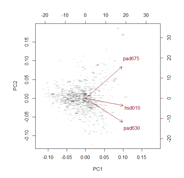
The example below shows a principle components analysis (PCA).
pc <- svyprcomp(~pad630+pad675+hsd010, design=nhc,scale=TRUE,scores=TRUE)
pc
Standard deviations (1, .., p=3):
[1] 1.3023573 0.8183481 0.7963491

Rotation (n x k) = (3 x 3):
          PC1          PC2          PC3
pad630    0.5769018    -0.5906013   -0.5642468
pad675    0.5690424     0.7861726   -0.2410879
hsd010    0.5859822    -0.1819963    0.7896216
biplot(pc, weight="scaled")
This is an example of Cronbach’s alpha.
svycralpha(~hsq571+dmdborn4, design=nhc, na.rm = TRUE)
*alpha*
0.1339271

