Chapter Outline
4.1 Robust Regression Methods
4.1.1 Regression with Robust Standard Errors
4.1.2 Using the Cluster Option
4.1.3 Robust Regression
4.1.4 Quantile Regression
4.2 Constrained Linear Regression
4.3 Regression with Censored or Truncated Data
4.3.1 Regression with Censored Data
4.3.2 Regression with Truncated Data
4.4 Multiple Equation Regression Models
4.4.1 Seemingly Unrelated Regression
4.4.2 Multivariate Regression
4.5 Summary
4.6 Self assessment
4.8 For more information
In this chapter we will go into various functions that go beyond OLS. This chapter is a bit different from the others in that it covers a number of different concepts, some of which may be new to you. These extensions, beyond OLS, have much of the look and feel of OLS but will provide you with additional tools to work with linear models.
The topics will include robust regression methods, constrained linear regression, regression with censored and truncated data, regression with measurement error, and multiple equation models.
4.1 Robust Regression Methods
It seems to be a rare dataset that meets all of the assumptions underlying multiple regression. We know that failure to meet assumptions can lead to biased estimates of coefficients and especially biased estimates of the standard errors. This fact explains a lot of the activity in the development of robust regression methods.
The idea behind robust regression methods is to make adjustments in the estimates that take into account some of the flaws in the data itself. We are going to look at three approaches to robust regression: 1) regression with robust standard errors including the cluster option, 2) robust regression using iteratively reweighted least squares, and 3) quantile regression, more specifically, median regression.
Before we look at these approaches, let’s look at a standard OLS regression using the elementary school academic performance index (elemapi2.dta) dataset.
setwd("D:DATA_stata8statawebbooksreg")
library(foreign)
api<-read.dta("elemapi2.dta")
Warning message:
value labels (dname) for dnum are missing in: read.dta("elemapi2.dta")
We will look at a model that predicts the api 2000 scores using the average class size in K through 3 (acs.k3), average class size 4 through 6 (acs.46), the percent of fully credentialed teachers (full), and the size of the school (enroll). First let’s look at the descriptive statistics for these variables. Note the missing values for acs.k3 and acs.k6.
 attach(api)
 myvar<-cbind(api00, acs.k3, acs.46, full, enroll)
 summary(myvar)
     api00           acs.k3          acs.46           full            enroll
 Min.   :369.0   Min.   :14.00   Min.   :20.00   Min.   : 37.00   Min.   : 130.0
 1st Qu.:523.8   1st Qu.:18.00   1st Qu.:27.00   1st Qu.: 76.00   1st Qu.: 320.0
 Median :643.0   Median :19.00   Median :29.00   Median : 88.00   Median : 435.0
 Mean   :647.6   Mean   :19.16   Mean   :29.69   Mean   : 84.55   Mean   : 483.5
 3rd Qu.:762.3   3rd Qu.:20.00   3rd Qu.:31.00   3rd Qu.: 97.00   3rd Qu.: 608.0
 Max.   :940.0   Max.   :25.00   Max.   :50.00   Max.   :100.00   Max.   :1570.0
                 NA's   : 2.00   NA's   : 3.00
Below we see the regression predicting api00 from acs.k3, acs.46 full and enroll. We see that all of the variables are significant except for acs.k3.
rm1<-lm(api00 ~ acs.k3 + acs.46 + full + enroll, api)
summary(rm1)
Residuals: Min 1Q Median 3Q Max -284.751 -80.076 -1.667 88.007 279.806Coefficients: Estimate Std. Error t value Pr(>|t|) (Intercept) -5.20041 84.95492 -0.061 0.951220 acs.k3 6.95438 4.37110 1.591 0.112422 acs.46 5.96601 1.53105 3.897 0.000115 *** full 4.66822 0.41425 11.269 < 2e-16 *** enroll -0.10599 0.02695 -3.932 9.96e-05 *** --- Signif. codes: 0 `***' 0.001 `**' 0.01 `*' 0.05 `.' 0.1 ` ' 1Residual standard error: 112.2 on 390 degrees of freedom Multiple R-Squared: 0.3849, Adjusted R-squared: 0.3786 F-statistic: 61.01 on 4 and 390 DF, p-value: < 2.2e-16
We can use the anova function to test both of the class size variables, and we find the overall test of these two variables is significant.
attach(api) api$ok <-complete.cases(api00, acs.k3, acs.46, full, enroll) api2<-api[api$ok,] rm1<-lm(api00 ~ acs.k3 + acs.46 + full + enroll, api2) rm2<-lm(api00 ~ full + enroll, api2) anova(rm2, rm1)Analysis of Variance TableModel 1: api00 ~ full + enroll Model 2: api00 ~ acs.k3 + acs.46 + full + enroll Res.Df RSS Df Sum of Sq F Pr(>F) 1 392 5188375 2 390 4909501 2 278874 11.077 2.095e-05 *** --- Signif. codes: 0 `***' 0.001 `**' 0.01 `*' 0.05 `.' 0.1 ` ' 1
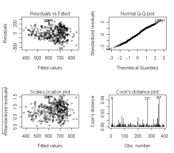
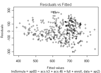
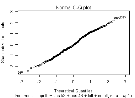
Here is a sequence of diagnostics plots for this regression.
plot(rm1)
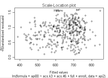
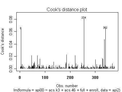
we use the avp function to plot a sequence of added variable plots. Notice that function avp is interactive. You first choose a variable to plot and then right click on the plot to stop it to continue to next plot.
avp(rm1)1:(Intercept) 2:acs.k3 3:acs.46 4:full 5:enroll Selection: 2
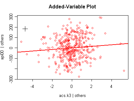
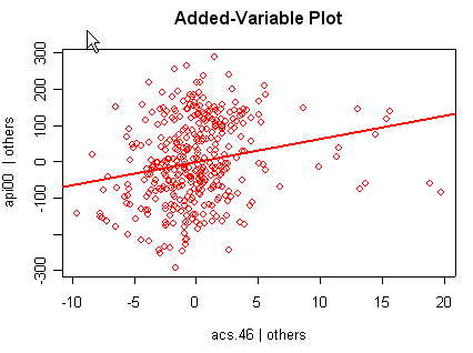
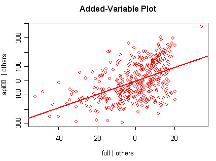
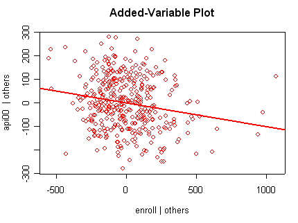
There is not a single extreme point (like we saw in chapter
2)
but a handful of points that stick out. For example, in the top right graph you can
see a handful of points that stick out from the rest. If this were just one or two
points, we might look for mistakes or for outliers, but we would be more reluctant to
consider such a large number of points as outliers.
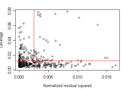
We can also plot the leverage against the squared residuals. To this end, we will create a variable of the normalized residual squared and the variable of leverage. We see 4 points that are somewhat high in both their leverage and their residuals.
m1<-lm(api00~acs.k3 + acs.46 + full + enroll, api) res<-m1$residuals res2<-res*res d<-sum(res2) res2<-res2/d h<-hatvalues(m1) x<-1/length(res2) y<-m1$rank*x plot(res2, h, xlab="Normalized residual squared", ylab="Leverage") abline(h=y, col="red") abline(v=x, col="red")
None of these results are dramatic problems, but the residual vs. fitted plot suggests that there might be some outliers and some possible heteroscedasticity; the avp plots have some observations that look to have high leverage, and the leverage vs. normalized residual squared shows some points in the upper right quadrant that could be influential. We might wish to use something other than OLS regression to estimate this model. In the next several sections we will look at some robust regression methods.
4.1.1 Regression with Robust Standard Errors
The R function robcov in Design package after the OLS regression model will give us the estimates of robust standard error. It implements two different ways of estimation: using the Huber-White sandwich estimators and Enfron’s method. Such robust standard errors can deal with a collection of minor concerns about failure to meet assumptions, such as minor problems about normality, heteroscedasticity, or some observations that exhibit large residuals, leverage or influence. For such minor problems, the robust standard errors may effectively deal with these concerns.
With the robcov function, the point estimates of the coefficients are exactly the same as in ordinary OLS, but the standard errors take into account issues concerning heterogeneity and lack of normality. Function robcov takes an object created by ols function which is also included in Design package. Note the changes in the standard errors and t-tests (but no change in the coefficients). In this particular example, using robust standard errors did not change any of the conclusions from the original OLS regression.
library(Design) m1<-ols(api00~acs.k3 + acs.46 + full + enroll, api, x=T, y=T) robcov(m1)
Linear Regression Model
ols(formula = api00 ~ acs.k3 + acs.46 + full + enroll, data = api,
x = T, y = T)
Frequencies of Missing Values Due to Each Variable
api00 acs.k3 acs.46 full enroll
0 2 3 0 0
n Model L.R. d.f. R2 Sigma
395 191.9 4 0.3849 112.2
Residuals:
     Min       1Q   Median       3Q      Max
-284.751  -80.076   -1.667   88.007  279.806
Coefficients:
           Value Std. Error        t  Pr(>|t|)
Intercept -5.200   86.11283 -0.06039 0.9518755
acs.k3     6.954    4.59126  1.51470 0.1306586
acs.46     5.966    1.56323  3.81648 0.0001574
full       4.668    0.41205 11.32930 0.0000000
enroll    -0.106    0.02784 -3.80748 0.0001630
Residual standard error: 112.2 on 390 degrees of freedom
Adjusted R-Squared: 0.3786
4.1.2 Using the Cluster Option
As described in Chapter 2, OLS regression assumes that the residuals are independent. The elemapi2 dataset contains data on 400 schools that come from 37 school districts. It is very possible that the scores within each school district may not be independent, and this could lead to residuals that are not independent within districts. In function robcov, we can use the cluster option to indicate that the observations are clustered into districts (based on dnum) and that the observations may be correlated within districts, but would be independent between districts.
Now, we can run robcov with the cluster option. Note that the standard errors have changed substantially, much more so, than the change caused by the robcov itself.
library(Design)
m1<-ols(api00~acs.k3 + acs.46 + full + enroll, api, x=T, y=T)
robcov(m1, cluster=dnum)
Linear Regression Modelols(formula = api00 ~ acs.k3 + acs.46 + full + enroll, data = api, x = T, y = T)Frequencies of Missing Values Due to Each Variable api00 acs.k3 acs.46 full enroll 0 2 3 0 0n Model L.R. d.f. R2 Sigma 395 191.9 4 0.3849 112.2Residuals: Min 1Q Median 3Q Max -284.751 -80.076 -1.667 88.007 279.806Coefficients: Value Std. Error t Pr(>|t|) Intercept -5.200 119.51722 -0.04351 9.653e-01 acs.k3 6.954 6.77258 1.02684 3.051e-01 acs.46 5.966 2.48393 2.40184 1.678e-02 full 4.668 0.69036 6.76200 4.988e-11 enroll -0.106 0.04215 -2.51474 1.231e-02Residual standard error: 112.2 on 390 degrees of freedom Adjusted R-Squared: 0.3786
As with the robcov without the cluster option, the estimate of the coefficients are the same as the OLS estimates, but the standard errors take into account that the observations within districts are non-independent. Even though the standard errors are larger in this analysis, the three variables that were significant in the OLS analysis are significant in this analysis as well. These standard errors are computed based on aggregate scores for the 37 districts, since these district level scores should be independent. If you have a very small number of clusters compared to your overall sample size it is possible that the standard errors could be quite larger than the OLS results. For example, if there were only 3 districts, the standard errors would be computed on the aggregate scores for just 3 districts.
4.1.3 Robust Regression
R has a few functions that performs robust regression using iteratively reweighted least squares. In fact, extremely deviant cases, those with Cook’s D greater than 1, can have their weights set to missing so that they are not included in the analysis at all.
We will use rlm function in MASS package. Note that in this analysis both the coefficients and the standard errors differ from the original OLS regression.
attach(api)
api$ok<-complete.cases(api00, acs.k3, acs.46, full, enroll)
api2<-api[ok,]
api2<-api[api$ok,]
detach(api)
attach(api2)
rrm1<-rlm(api00 ~ acs.k3 + acs.46 + full + enroll, api2, psi = psi.bisquare)
summary(rrm1)
Call: rlm(formula = api00 ~ acs.k3 + acs.46 + full + enroll, data = api2, psi = psi.bisquare) Residuals: Min 1Q Median 3Q Max -286.122 -81.508 -2.010 87.636 280.456Coefficients: Value Std. Error t value (Intercept) -6.7777 90.2148 -0.0751 acs.k3 6.1253 4.6417 1.3196 acs.46 6.2507 1.6258 3.8446 full 4.7936 0.4399 10.8971 enroll -0.1092 0.0286 -3.8148Residual standard error: 122.2 on 390 degrees of freedomCorrelation of Coefficients:(Intercept) acs.k3 acs.46 full acs.k3 -0.7530 acs.46 -0.2498 -0.2480 full -0.2421 -0.1824 -0.0871 enroll -0.1277 -0.1623 -0.0304 0.3638
If you compare the robust regression results (directly above) with the OLS results previously presented, you can see that the coefficients and standard errors are quite similar, and the t values and p values are also quite similar. Despite the minor problems that we found in the data when we performed the OLS analysis, the robust regression analysis yielded quite similar results suggesting that indeed these were minor problems. Had the results been substantially different, we would have wanted to further investigate the reasons why the OLS and robust regression results were different, and among the two results the robust regression results would probably be the more trustworthy.
Let’s look at the predicted (fitted) values (p), the residuals (r), the leverage (hat) values (h) and the final weight used in the regression analysis.
names(rrm1)
 [1] "coefficients"  "residuals"     "effects"       "rank"
 [5] "fitted.values" "assign"        "qr"            "df.residual"
 [9] "w"             "s"             "psi"           "k2"
[13] "weights"       "conv"          "converged"     "x"
[17] "call"          "terms"         "xlevels"       "model"
h<-hatvalues(rrm1) a<-cbind(snum=api2$snum, api00 = api2$api00, p=as.list(rrm1$fitted.values), r=as.list(rrm1$residuals), h=h, wgt=rrm1$w)head(a) snum api00 p r h wgt 1 906 693 566.0879 126.9121 0.02255447 0.9040987 2 889 570 613.2651 -43.26507 0.03357404 0.9886118 3 887 546 536.4558 9.544233 0.01383015 0.999444 4 876 571 674.6527 -103.6527 0.003933971 0.9354946 5 888 478 657.5154 -179.5154 0.005021648 0.812976 6 4284 858 763.9115 94.08854 0.007430161 0.9466887
Now, let’s check on the various predicted values and the weighting. First, we will sort by wgt then we will look at the first 15 observations. Notice that the smallest weights are near one-half but quickly get into the .7 range.
a.st<-a[order(as.numeric(wgt)),]head(a.st, n=10) snum api00 p r h wgt 64 637 447 733.1216 -286.1216 0.00384723 0.5627222 339 5387 892 611.5442 280.4558 0.002390878 0.5775071 239 2267 897 621.5446 275.4554 0.01042099 0.5904899 56 65 903 631.3234 271.6766 0.01077368 0.6002285 274 3759 585 842.4706 -257.4706 0.04253686 0.6362807 392 5926 469 715.1664 -246.1664 0.005898797 0.6643258 196 1978 894 650.776 243.224 0.005960851 0.6714925 249 3696 483 721.2649 -238.2649 0.00531516 0.6834994 44 5222 940 707.623 232.3771 0.004179216 0.697546 67 690 424 654.532 -230.5320 0.009411466 0.7019176
Now, let’s look at the last 10 observations. The weights for observations 391 to 395 are all very close to one. The values for observations 396 to the end are missing due to the missing predictors. Note that the observations above that have the lowest weights are also those with the largest residuals (residuals over 200) and the observations below with the highest weights have very low residuals (all less than 3).
tail(a.st, n=10)
    snum api00 p        r          h           wgt
390 5917 735   730.9272 4.072759   0.006123765 0.9998986
169 1949 696   691.9574 4.042584   0.02132037  0.9998998
235 181  724   727.5296 -3.529599  0.01430605  0.9999239
155 1596 536   533.285  2.714995   0.01272140  0.9999551
252 3700 717   719.4086 -2.408607  0.007685493 0.9999647
76  3024 727   729.0097 -2.009694  0.01064497  0.9999754
262 3535 705   703.8085 1.191496   0.004877017 0.9999913
127 1885 605   605.407  -0.4069951 0.01432873  0.999999
298 4486 706   705.8076 0.1923886  0.01447260  0.9999998
187 1678 497   496.876  0.1240031  0.02404090  1
After using rlm, it is possible to generate diagnostics plots just as we have seen for OLS regression.
op <- par(mfrow=c(2,2), cex=.9, omi=c(.1, .1, .1, .1))
plot(rrm1, ask=F)
par(op)
4.1.4 Quantile Regression
Quantile regression, in general, and median regression, in particular, might be considered as an alternative to rlm. The R package quantreg offers functions for quantile regression. We will have to install the package and load it before using any functions of the package. Function we are going to use is rq and without any options it will actually do a median regression in which the coefficients will be estimated by minimizing the absolute deviations from the median. Of course, as an estimate of central tendency, the median is a resistant measure that is not as greatly affected by outliers as is the mean. It is not clear that median regression is a resistant estimation procedure, in fact, there is some evidence that it can be affected by high leverage values.
Here is what the quantile regression looks like using rq function. The coefficient and standard error for acs.k3 are considerably different when using rq as compared to OLS using the lm function (the coefficients are 1.2 vs 6.9 and the standard errors are 6.4 vs 4.3). The coefficients and standard errors for the other variables are also different, but not as dramatically different. Nevertheless, the rq results indicate that, like the OLS results, all of the variables except acs.k3 are significant.
install.packages("quantreg")
library(quantreg)
rrm2<-rq(api00 ~ acs.k3 + acs.46 + full + enroll, data=api2, method="fn")
summary(rrm2, se="ker")
Call: rq(formula = api00 ~ acs.k3 + acs.46 + full + enroll, data = api2, method = "fn")tau: [1] 0.5Coefficients: Value Std. Error t value Pr(>|t|) (Intercept) 17.1505 132.7689 0.1292 0.8973 acs.k3 1.2691 6.9169 0.1835 0.8545 acs.46 7.2241 2.5879 2.7915 0.0055 full 5.3238 0.7056 7.5448 0.0000 enroll -0.1246 0.0449 -2.7769 0.0057
There are a few different methods implemented for rq function. We used method="fn" which stands for Frisch Newton interior point method. The default method is method="br" which is a modified version of the Barrodale and Roberts algorithm for l1-regression. There are also a couple of ways of estimating the standard errors. We used se = "ker" fo kernel estimate of the sandwich. One can also use se = "boot" for bootstrapping method for estimating standard errors.
4.2 Constrained Linear Regression
Let’s begin this section by looking at a regression model using the hsb2 dataset. The hsb2 file is a sample of 200 cases from the Highschool and Beyond Study (Rock, Hilton, Pollack, Ekstrom & Goertz, 1985). It includes the following variables: id, female, race, ses, schtyp, program, read, write, math, science and socst. The variables read, write, math, science and socst are the results of standardized tests on reading, writing, math, science and social studies (respectively), and the variable female is coded 1 if female, 0 if male.
library(foreign)
hsb2<-read.dta("hsb2.dta")
summary(hsb2)
       id            female              race         ses         schtyp
 Min.   :  1.00   male  : 91   hispanic    : 24   low   :47   public :168
 1st Qu.: 50.75   female:109   asian       : 11   middle:95   private: 32
 Median :100.50                african-amer: 20   high  :58
 Mean   :100.50                white       :145
 3rd Qu.:150.25
 Max.   :200.00
       prog          read           write            math          science
 general : 45   Min.   :28.00   Min.   :31.00   Min.   :33.00   Min.   :26.00
 academic:105   1st Qu.:44.00   1st Qu.:45.75   1st Qu.:45.00   1st Qu.:44.00
 vocation: 50   Median :50.00   Median :54.00   Median :52.00   Median :53.00
                Mean   :52.23   Mean   :52.77   Mean   :52.65   Mean   :51.85
                3rd Qu.:60.00   3rd Qu.:60.00   3rd Qu.:59.00   3rd Qu.:58.00
                Max.   :76.00   Max.   :67.00   Max.   :75.00   Max.   :74.00
     socst
 Min.   :26.0
 1st Qu.:46.0
 Median :52.0
 Mean   :52.4
 3rd Qu.:61.0
 Max.   :71.0
Let’s start by doing an OLS regression where we predict socst score from read, write, math, science and female (gender)
m1<-lm(socst ~ read + write + math + science + female)
summary(m1)
Residuals:
    Min      1Q  Median      3Q     Max
-22.337  -5.729   1.011   5.390  17.206
Coefficients:
             Estimate Std. Error t value Pr(>|t|)
(Intercept)   7.33934    3.65024   2.011   0.0457 *
read          0.37840    0.08063   4.693 5.07e-06 ***
write         0.38587    0.08893   4.339 2.30e-05 ***
math          0.13033    0.08938   1.458   0.1464
science      -0.03339    0.08187  -0.408   0.6838
femalefemale -0.35326    1.24537  -0.284   0.7770
---
Signif. codes:  0 `***' 0.001 `**' 0.01 `*' 0.05 `.' 0.1 ` ' 1
Residual standard error: 7.861 on 194 degrees of freedom
Multiple R-Squared: 0.4774,     Adjusted R-squared: 0.4639
F-statistic: 35.44 on 5 and 194 DF,  p-value: < 2.2e-16
Notice that the coefficients for read and write are very similar, which makes sense since they are both measures of language ability. Also, the coefficients for math and science are similar (in that they are both not significantly different from 0). Suppose that we have a theory that suggests that read and write should have equal coefficients, and that math and science should have equal coefficients as well. We can test the equality of the coefficients using the anova function.
m1a<-lm(socst ~ I(read + write) + math + science + female)
anova(m1a, m1)
Analysis of Variance Table
Model 1: socst ~ I(read + write) + math + science + female Model 2: socst ~ read + write + math + science + female Res.Df RSS Df Sum of Sq F Pr(>F) 1 195 11987.1 2 194 11986.9 1 0.2 0.0031 0.9558
The result indicates that there is no significant difference in the coefficients for the reading and writing scores. Since it appears that the coefficients for math and science are also equal, let’s test the equality of those as well.
m1b<-lm(socst ~ read + write + I(math + science) + female)
anova(m1b, m1)
Analysis of Variance Table
Model 1: socst ~ read + write + I(math + science) + female Model 2: socst ~ read + write + math + science + female Res.Df RSS Df Sum of Sq F Pr(>F) 1 195 12076.6 2 194 11986.9 1 89.6 1.4508 0.2299
Let’s now perform both of these tests together, simultaneously testing that the coefficient for read equals write and math equals science.
m1c<-lm(socst ~ I(read + write) + I(math + science) + female)
anova(m1c, m1)
Analysis of Variance Table
Model 1: socst ~ I(read + write) + I(math + science) + female Model 2: socst ~ read + write + math + science + female Res.Df RSS Df Sum of Sq F Pr(>F) 1 196 12076.6 2 194 11986.9 2 89.7 0.7259 0.4852
Note this second test has 2 df, since it is testing both of the hypotheses listed, and this test is not significant, suggesting these pairs of coefficients are not significantly different from each other. We can estimate regression models where we constrain coefficients to be equal to each other. For example, we have already constrained the effects of read to equal write to be eqaul in model m1a.
summary(m1a)Call: lm(formula = socst ~ I(read + write) + math + science + female)Residuals: Min 1Q Median 3Q Max -22.304 -5.762 1.019 5.411 17.176Coefficients: Estimate Std. Error t value Pr(>|t|) (Intercept) 7.35415 3.63118 2.025 0.0442 * I(read + write) 0.38185 0.05139 7.430 3.32e-12 *** math 0.13030 0.08915 1.462 0.1454 science -0.03328 0.08164 -0.408 0.6840 femalefemale -0.32962 1.16736 -0.282 0.7780 --- Signif. codes: 0 `***' 0.001 `**' 0.01 `*' 0.05 `.' 0.1 ` ' 1Residual standard error: 7.84 on 195 degrees of freedom Multiple R-Squared: 0.4774, Adjusted R-squared: 0.4667 F-statistic: 44.53 on 4 and 195 DF, p-value: < 2.2e-16
Notice that the coefficients for read and write are identical, along with their standard errors, t-test, etc. Also note that the degrees of freedom for the F test is four, not five, as in the OLS model. This is because only one coefficient is estimated for read and write, estimated like a single variable equal to the sum of their values. Notice also that the Root MSE is slightly higher for the constrained model, but only slightly higher (from the test comparing model m1 and m1a). This is because we have forced the model to estimate the coefficients for read and write that are not as good at minimizing the Sum of Squares Error (the coefficients that would minimize the SSE would be the coefficients from the unconstrained model).
Next, let us look at our model m1c where we constrain both read equal to write and math equal to science.
summary(m1c)Call: lm(formula = socst ~ I(read + write) + I(math + science) + female)Residuals: Min 1Q Median 3Q Max -23.650 -5.681 1.313 5.610 17.098Coefficients: Estimate Std. Error t value Pr(>|t|) (Intercept) 7.50566 3.63323 2.066 0.0402 * I(read + write) 0.38604 0.05133 7.520 1.92e-12 *** I(math + science) 0.04281 0.05192 0.824 0.4107 femalefemale -0.20087 1.16383 -0.173 0.8631 --- Signif. codes: 0 `***' 0.001 `**' 0.01 `*' 0.05 `.' 0.1 ` ' 1Residual standard error: 7.85 on 196 degrees of freedom Multiple R-Squared: 0.4735, Adjusted R-squared: 0.4654 F-statistic: 58.75 on 3 and 196 DF, p-value: < 2.2e-16anova(m1c, m1b) Analysis of Variance TableModel 1: socst ~ I(read + write) + I(math + science) + female Model 2: socst ~ read + write + I(math + science) + female Res.Df RSS Df Sum of Sq F Pr(>F) 1 196 12076.6 2 195 12076.6 1 0.1 0.0011 0.9734
Now the coefficients for read = write and math = science and the degrees of freedom for the model has dropped to three. Again, the Root MSE is slightly larger than in the prior model, but we should emphasize only very slightly larger. If indeed the population coefficients for read = write and math = science, then these combined (constrained) estimates may be more stable and generalize better to other samples. So although these estimates may lead to slightly higher standard error of prediction in this sample, they may generalize better to the population from which they came.
4.3 Regression with Censored or Truncated Data
Analyzing data that contain censored values or are truncated is common in many research disciplines. According to Hosmer and Lemeshow (1999), a censored value is one whose value is incomplete due to random factors for each subject. A truncated observation, on the other hand, is one which is incomplete due to a selection process in the design of the study.
We will begin by looking at analyzing data with censored values.
4.3.1 Regression with Censored Data
In this example we have a variable called acadindx which is a weighted combination of standardized test scores and academic grades. The maximum possible score on acadindx is 200 but it is clear that the 16 students who scored 200 are not exactly equal in their academic abilities. In other words, there is variability in academic ability that is not being accounted for when students score 200 on acadindx. The variable acadindx is said to be censored, in particular, it is right censored.
Let’s look at the example. We will begin by looking at a description of the data, some descriptive statistics, and correlations among the variables.
library(foreign)
acind<-read.dta("acadindx.dta")
attach(acind)
head(acind)
  id female reading writing acadindx
1  1 female      34      44      147
2  2 female      39      41      143
3  3   male      63      65      179
4  4 female      44      50      148
5  5   male      47      40      156
6  6 female      47      41      154
summary(acind)
       id            female       reading         writing         acadindx
 Min.   :  1.00   male  : 91   Min.   :28.00   Min.   :31.00   Min.   :138.0
 1st Qu.: 50.75   female:109   1st Qu.:44.00   1st Qu.:45.75   1st Qu.:158.8
 Median :100.50                Median :50.00   Median :54.00   Median :172.0
 Mean   :100.50                Mean   :52.23   Mean   :52.77   Mean   :172.2
 3rd Qu.:150.25                3rd Qu.:60.00   3rd Qu.:60.00   3rd Qu.:184.3
 Max.   :200.00                Max.   :76.00   Max.   :67.00   Max.   :200.0
nrow(acind)
[1] 200
a<-cbind(acadindx, female=as.numeric(female), reading, writing)
cor(a)
            acadindx      female     reading   writing
acadindx  1.00000000 -0.08209921  0.71309434 0.6625551
female   -0.08209921  1.00000000 -0.05308387 0.2564915
reading   0.71309434 -0.05308387  1.00000000 0.5967765
writing   0.66255508  0.25649154  0.59677648 1.0000000
Now, let’s run a standard OLS regression on the data and generate predicted scores in p1.
m0<-lm(acadindx ~ factor(female) + reading + writing)
summary(m0)
Call:
lm(formula = acadindx ~ factor(female) + reading + writing)
Residuals:
       Min         1Q     Median         3Q        Max
-26.066904  -6.711611   0.002891   6.364159  38.294667
Coefficients:
                     Estimate Std. Error t value Pr(>|t|)
(Intercept)          96.11841    4.48956  21.409  < 2e-16 ***
factor(female)female -5.83250    1.58821  -3.672  0.00031 ***
reading               0.71842    0.09315   7.713 6.09e-13 ***
writing               0.79057    0.10410   7.594 1.24e-12 ***
---
Signif. codes:  0 `***' 0.001 `**' 0.01 `*' 0.05 `.' 0.1 ` ' 1
Residual standard error: 10.42 on 196 degrees of freedom
Multiple R-Squared: 0.6218,     Adjusted R-squared: 0.616
F-statistic: 107.4 on 3 and 196 DF,  p-value: < 2.2e-16
p1<-m0$fitted.values
head(p1)
       1        2        3        4        5        6
149.4972 150.7176 192.7658 161.4248 161.5068 156.4649
is.list(p1)
[1] FALSE
is.vector(p1)
[1] TRUE
The tobit model in R can be estimated using the survreg function from survival package with Gaussian distribution. We will follow the tobit mdoel by predicting p2 containing the tobit predicted values.
library(survival)
tm1 <-survreg(Surv(acadindx, acadindx<200, type='right') ~
             factor(female) + reading + writing, data=acind, dist='gaussian')
summary(tm1)
Call:
survreg(formula = Surv(acadindx, acadindx < 200, type = "right") ~
    factor(female) + reading + writing, data = acind, dist = "gaussian")
                      Value Std. Error     z        p
(Intercept)          92.738     4.8034 19.31 4.73e-83
factor(female)female -6.347     1.6924 -3.75 1.77e-04
reading               0.778     0.0997  7.80 6.15e-15
writing               0.811     0.1102  7.36 1.84e-13
Log(scale)            2.397     0.0529 45.28 0.00e+00
Scale= 11
Gaussian distribution
Loglik(model)= -718.1   Loglik(intercept only)= -813.3
        Chisq= 190.39 on 3 degrees of freedom, p= 0
Number of Newton-Raphson Iterations: 6
n= 200
names(tm1)
 [1] "coefficients"      "icoef"             "var"
 [4] "loglik"            "iter"              "linear.predictors"
 [7] "df"                "scale"             "idf"
[10] "df.residual"       "terms"             "means"
[13] "call"              "dist"              "y"
p2<-tm1$linear.predictors
Summarizing the p1 and p2 scores shows that the tobit predicted values have a greater range of values.
summary(cbind(p1, p2, acadindx))
       p1              p2           acadindx
 Min.   :142.4   Min.   :141.2   Min.   :138.0
 1st Qu.:161.5   1st Qu.:161.6   1st Qu.:158.8
 Median :172.4   Median :172.9   Median :172.0
 Mean   :172.2   Mean   :172.7   Mean   :172.2
 3rd Qu.:182.3   3rd Qu.:183.3   3rd Qu.:184.3
 Max.   :201.5   Max.   :203.9   Max.   :200.0
When we look at a listing of p1 and p2 for all students who scored the maximum of 200 on acadindx, we see that in every case the tobit predicted value is greater than the OLS predicted value. These predictions represent an estimate of what the variability would be if the values of acadindx could exceed 200.
(cbind(p1, p2, acadindx)[acadindx==200,])
          p1       p2 acadindx
32  179.1750 179.6200      200
57  192.6806 194.3291      200
68  201.5311 203.8541      200
80  191.8309 193.5770      200
82  188.1537 189.5627      200
88  186.5725 187.9405      200
95  195.9971 198.1762      200
100 186.9333 188.1076      200
132 197.5783 199.7984      200
136 189.4592 191.1436      200
143 191.1847 192.8327      200
157 191.6145 193.4767      200
161 180.2511 181.0082      200
169 182.2750 183.3667      200
174 191.6145 193.4767      200
200 187.6616 189.4210      200
4.3.2 Regression with Truncated Data
Truncated data occurs when some observations are not included in the analysis because of the value of the variable. We will illustrate analysis with truncation using the dataset, acadindx, that was used in the previous section. If acadindx is no longer loaded in memory you can get it with the following use command.
library(foreign)
acind<-read.dta("acadindx.dta")
attach(acind)
Let’s imagine that in order to get into a special honors program, students need to score at least 160 on acadindx. So we will drop all observations in which the value of acadindx is less than 160.
acind160<-acind[acadindx>160,]
Now, let’s estimate the same model that we used in the section on censored data, only this time we will pretend that a 200 for acadindx is not censored.
cm1<-lm(acadindx ~ factor(female) + reading + writing, data = acind160)
summary(cm1)
Call: lm(formula = acadindx ~ factor(female) + reading + writing, data = acind160)Residuals: Min 1Q Median 3Q Max -20.9569 -6.7716 -0.1888 5.7004 28.7576Coefficients: Estimate Std. Error t value Pr(>|t|) (Intercept) 125.63547 5.89156 21.325 < 2e-16 *** factor(female)female -5.23849 1.61563 -3.242 0.00148 ** reading 0.44111 0.09635 4.578 1.03e-05 *** writing 0.58733 0.11508 5.104 1.07e-06 *** --- Signif. codes: 0 `***' 0.001 `**' 0.01 `*' 0.05 `.' 0.1 ` ' 1Residual standard error: 9.03 on 140 degrees of freedom Multiple R-Squared: 0.4143, Adjusted R-squared: 0.4017 F-statistic: 33.01 on 3 and 140 DF, p-value: 3.377e-16
4.4 Multiple Equation Regression Models
If a dataset has enough variables we may want to estimate more than one regression model. For example, we may want to predict y1 from x1 and also predict y2 from x2. Even though there are no variables in common these two models are not independent of one another because the data come from the same subjects. This is an example of one type of multiple equation regression known as seemingly unrelated regression. We can estimate the coefficients and obtain standard errors taking into account the correlated errors in the two models. An important feature of multiple equation models is that we can test predictors across equations.
Another example of multiple equation regression is if we wished to predict y1, y2 and y3 from x1 and x2. This is a three equation system, known as multivariate regression, with the same predictor variables for each model. Again, we have the capability of testing coefficients across the different equations.
Multiple equation models are a powerful extension to our data analysis tool kit.
4.4.1 Seemingly Unrelated Regression
Let’s continue using the hsb2 data file to illustrate the use of seemingly unrelated regression. You can load it into memory again if it has been cleared out.
hsb2<-read.dta("hsb2.dta")
attach(hsb2)
This time let’s look at two regression models.
    science = math female
    write   = read female
It is the case that the errors (residuals) from these two models would be correlated. This would be true even if the predictor female were not found in both models. The errors would be correlated because all of the values of the variables are collected on the same set of observations. This is a situation tailor made for seemingly unrelated regression. A recent R package systemfit can be used for estimation of seemingly unrelated regression. You will have to download the package from CRAN and load it into memory.
install.packages("systemfit")
library(systemfit)
Here is our first model using OLS.
m1<-lm(science ~ math + female)
summary(m1)
Call: lm(formula = science ~ math + female)Residuals: Min 1Q Median 3Q Max -21.2985 -4.2885 0.1747 4.4511 24.6702Coefficients: Estimate Std. Error t value Pr(>|t|) (Intercept) 18.11813 3.16713 5.721 3.9e-08 *** math 0.66319 0.05787 11.460 < 2e-16 *** femalefemale -2.16840 1.08604 -1.997 0.0472 * --- Signif. codes: 0 `***' 0.001 `**' 0.01 `*' 0.05 `.' 0.1 ` ' 1Residual standard error: 7.645 on 197 degrees of freedom Multiple R-Squared: 0.4098, Adjusted R-squared: 0.4038 F-statistic: 68.38 on 2 and 197 DF, p-value: < 2.2e-16And here is our second model using OLS.
m2<-lm(write ~ read + female)
summary(m2)
Call: lm(formula = write ~ read + female)Residuals: Min 1Q Median 3Q Max -17.5227 -5.6580 0.1680 5.0435 15.1749Coefficients: Estimate Std. Error t value Pr(>|t|) (Intercept) 20.22837 2.71376 7.454 2.80e-12 *** read 0.56589 0.04938 11.459 < 2e-16 *** femalefemale 5.48689 1.01426 5.410 1.82e-07 *** --- Signif. codes: 0 `***' 0.001 `**' 0.01 `*' 0.05 `.' 0.1 ` ' 1Residual standard error: 7.133 on 197 degrees of freedom Multiple R-Squared: 0.4394, Adjusted R-squared: 0.4337 F-statistic: 77.21 on 2 and 197 DF, p-value: < 2.2e-16
With the function systemfit we can estimate both models simultaneously while accounting for the correlated errors at the same time, leading to efficient estimates of the coefficients and standard errors.
eq1 <- science ~ math + female
eq2  <- write ~ read + female
labels <- list( "eq1", "eq2" )
system <- list( eq1, eq2 )

fitsur <- systemfit("SUR", system, labels, data=hsb2 )
print( fitsur )
systemfit results method: SURN DF SSR MSE RMSE R2 Adj R2 eq1 200 197 11539.2 58.5747 7.65341 0.408473 0.402468 eq2 200 197 10041.8 50.9738 7.13959 0.438341 0.432639The covariance matrix of the residuals used for estimation eq1 eq2 eq1 58.44645 7.89076 eq2 7.89076 50.87591The covariance matrix of the residuals eq1 eq2 eq1 58.57469 9.36845 eq2 9.36845 50.97379The correlations of the residuals eq1 eq2 eq1 1.000000 0.171451 eq2 0.171451 1.000000The determinant of the residual covariance matrix: 2898.01 OLS R-squared value of the system: 0.422756 McElroy's R-squared value for the system: 0.380127SUR estimates for eq1 (equation 1 ) Model Formula: science ~ math + femaleEstimate Std. Error t value Pr(>|t|) (Intercept) 20.132648 3.149485 6.392361 0 *** math 0.625141 0.057528 10.866753 0 *** femalefemale -2.189344 1.086038 -2.015901 0.045169 * --- Signif. codes: 0 `***' 0.001 `**' 0.01 `*' 0.05 `.' 0.1 ` ' 1Residual standard error: 7.65341 on 197 degrees of freedom Number of observations: 200 Degrees of Freedom: 197 SSR: 11539.214156 MSE: 58.574691 Root MSE: 7.65341 Multiple R-Squared: 0.408473 Adjusted R-Squared: 0.402468SUR estimates for eq2 (equation 2 ) Model Formula: write ~ read + femaleEstimate Std. Error t value Pr(>|t|) (Intercept) 21.834387 2.698827 8.090323 0 *** read 0.535484 0.049091 10.908024 0 *** femalefemale 5.453748 1.014244 5.377153 0 *** --- Signif. codes: 0 `***' 0.001 `**' 0.01 `*' 0.05 `.' 0.1 ` ' 1Residual standard error: 7.139593 on 197 degrees of freedom Number of observations: 200 Degrees of Freedom: 197 SSR: 10041.836153 MSE: 50.973788 Root MSE: 7.139593 Multiple R-Squared: 0.438341 Adjusted R-Squared: 0.432639
Now that we have estimated our models let’s test the predictor variables. The test for female combines information from both models. The function to do the test is lrtest.systemfit to perform loglikelihood ratio test. To test that the effect of female is zero is compare the model which includes female as a predictor and the model without female as a predictor.
eq1 <- science ~ math
eq2  <- write ~ read
labels <- list( "eq1", "eq2" )
system <- list( eq1, eq2 )
fitsur2 <- systemfit("SUR", system, labels, data=hsb2 ) lrtest.systemfit(fitsur2, fitsur)$df [1] 2$lr [1] 35.0$p [1] 2.46e-08
In the same way, we can also test on variable read and math. For example, we can test on the effect of math as shown below.
eq1 <- science ~ female
eq2  <- write ~ read + female
labels <- list( "eq1", "eq2" )
system <- list( eq1, eq2 )

fitsur3 <- systemfit("SUR", system, labels, data=hsb2 )
lrtest.systemfit(fitsur3, fitsur)
$df
[1] 1
$lr [1] 77.5$p [1] 0
Now, let’s estimate 3 models where we use the same predictors in each model as shown below.
     read  = female prog1 prog3
     write = female prog1 prog3
     math  = female prog1 prog3
Variable prog1 and prog3 are dummy variables for factor variable prog with its second category (academic) as the reference category.
table(prog)
prog
 general academic vocation
      45      105       50
hsb2$prog1<-prog=="general" hsb2$prog3<-prog=="vocation"
Let’s first estimate these three models using 3 OLS regressions.
m1 <-lm(read ~ female + prog1 + prog3, data=hsb2) summary(m1)Residuals: Min 1Q Median 3Q Max -22.830 -7.192 -0.126 6.795 22.356Coefficients: Estimate Std. Error t value Pr(>|t|) (Intercept) 56.83 1.17 48.55 < 2e-16 *** femalefemale -1.21 1.33 -0.91 0.36378 prog1TRUE -6.43 1.67 -3.86 0.00015 *** prog3TRUE -9.98 1.61 -6.21 3.1e-09 *** --- Signif. codes: 0 `***' 0.001 `**' 0.01 `*' 0.05 `.' 0.1 ` ' 1Residual standard error: 9.35 on 196 degrees of freedom Multiple R-Squared: 0.181, Adjusted R-squared: 0.169 F-statistic: 14.5 on 3 and 196 DF, p-value: 1.52e-08m2 <-lm(write ~ female + prog1 + prog3, data=hsb2) summary(m2)Call: lm(formula = write ~ female + prog1 + prog3, data = hsb2)Residuals: Min 1Q Median 3Q Max -21.393 -5.012 0.607 6.129 18.816Coefficients: Estimate Std. Error t value Pr(>|t|) (Intercept) 53.62 1.04 51.46 < 2e-16 *** femalefemale 4.77 1.18 4.04 7.8e-05 *** prog1TRUE -4.83 1.48 -3.26 0.0013 ** prog3TRUE -9.44 1.43 -6.60 3.8e-10 *** --- Signif. codes: 0 `***' 0.001 `**' 0.01 `*' 0.05 `.' 0.1 ` ' 1Residual standard error: 8.32 on 196 degrees of freedom Multiple R-Squared: 0.241, Adjusted R-squared: 0.229 F-statistic: 20.7 on 3 and 196 DF, p-value: 1.06e-11m3 <-lm(math ~ female + prog1 + prog3, data=hsb2) summary(m3)Residuals: Min 1Q Median 3Q Max -19.106 -6.727 -0.746 6.361 28.216Coefficients: Estimate Std. Error t value Pr(>|t|) (Intercept) 57.106 1.037 55.07 < 2e-16 *** femalefemale -0.674 1.176 -0.57 0.57 prog1TRUE -6.724 1.476 -4.56 9.1e-06 *** prog3TRUE -10.322 1.423 -7.25 9.2e-12 *** --- Signif. codes: 0 `***' 0.001 `**' 0.01 `*' 0.05 `.' 0.1 ` ' 1Residual standard error: 8.28 on 196 degrees of freedom Multiple R-Squared: 0.23, Adjusted R-squared: 0.219 F-statistic: 19.6 on 3 and 196 DF, p-value: 3.90e-11
These regressions provide fine estimates of the coefficients and standard errors but these results assume the residuals of each analysis are completely independent of the others. Also, if we wish to test female, we would have to do it three times and would not be able to combine the information from all three tests into a single overall test.
Now let’s use sur to estimate the same models.
eq1 <- read ~ female + prog1 + prog3 eq2 <- write ~ female + prog1 + prog3 eq3 <- math ~ female + prog1 + prog3 labels <- list( "eq1", "eq2", "eq3" ) system <- list( eq1, eq2, eq3 )fitsur <- systemfit("SUR", system, labels, data=hsb2 ) summary(fitsur)systemfit results method: SURN DF SSR MSE RMSE R2 Adj R2 eq1 200 196 17130.1 87.3987 9.34873 0.181137 0.168604 eq2 200 196 13574.5 69.2575 8.32211 0.240754 0.229132 eq3 200 196 13441.2 68.5775 8.28115 0.230428 0.218649The covariance matrix of the residuals used for estimation eq1 eq2 eq3 eq1 87.3987 42.9368 44.7051 eq2 42.9368 69.2575 38.4352 eq3 44.7051 38.4352 68.5775The covariance matrix of the residuals eq1 eq2 eq3 eq1 87.3987 42.9368 44.7051 eq2 42.9368 69.2575 38.4352 eq3 44.7051 38.4352 68.5775The correlations of the residuals eq1 eq2 eq3 eq1 1.000000 0.551878 0.577450 eq2 0.551878 1.000000 0.557705 eq3 0.577450 0.557705 1.000000The determinant of the residual covariance matrix: 168700 OLS R-squared value of the system: 0.215382 McElroy's R-squared value for the system: 0.152692SUR estimates for eq1 (equation 1 ) Model Formula: read ~ female + prog1 + prog3Estimate Std. Error t value Pr(>|t|) (Intercept) 56.829503 1.170562 48.548906 0 *** femalefemale -1.208582 1.327672 -0.910302 0.363781 prog1TRUE -6.42937 1.665893 -3.859413 0.000154 *** prog3TRUE -9.976868 1.606428 -6.210591 0 *** --- Signif. codes: 0 `***' 0.001 `**' 0.01 `*' 0.05 `.' 0.1 ` ' 1Residual standard error: 9.348725 on 196 degrees of freedom Number of observations: 200 Degrees of Freedom: 196 SSR: 17130.135878 MSE: 87.398652 Root MSE: 9.348725 Multiple R-Squared: 0.181137 Adjusted R-Squared: 0.168604SUR estimates for eq2 (equation 2 ) Model Formula: write ~ female + prog1 + prog3Estimate Std. Error t value Pr(>|t|) (Intercept) 53.621617 1.042019 51.459365 0 *** femalefemale 4.771211 1.181876 4.036981 7.8e-05 *** prog1TRUE -4.832929 1.482956 -3.258984 0.001318 ** prog3TRUE -9.438071 1.430021 -6.599953 0 *** --- Signif. codes: 0 `***' 0.001 `**' 0.01 `*' 0.05 `.' 0.1 ` ' 1Residual standard error: 8.32211 on 196 degrees of freedom Number of observations: 200 Degrees of Freedom: 196 SSR: 13574.472277 MSE: 69.257512 Root MSE: 8.32211 Multiple R-Squared: 0.240754 Adjusted R-Squared: 0.229132SUR estimates for eq3 (equation 3 ) Model Formula: math ~ female + prog1 + prog3Estimate Std. Error t value Pr(>|t|) (Intercept) 57.10551 1.03689 55.073828 0 *** femalefemale -0.673767 1.176059 -0.572903 0.567367 prog1TRUE -6.723945 1.475657 -4.556576 9e-06 *** prog3TRUE -10.321675 1.422983 -7.253549 0 *** --- Signif. codes: 0 `***' 0.001 `**' 0.01 `*' 0.05 `.' 0.1 ` ' 1Residual standard error: 8.281151 on 196 degrees of freedom Number of observations: 200 Degrees of Freedom: 196 SSR: 13441.182791 MSE: 68.577463 Root MSE: 8.281151 Multiple R-Squared: 0.230428 Adjusted R-Squared: 0.218649
In addition to getting more appropriate standard errors, sur allows us to test the effects of the predictors across the equations. We can test the hypothesis that the coefficient for female is 0 for all three outcome variables, as shown below.
eq1 <- read ~ prog1 + prog3 eq2 <- write ~ prog1 + prog3 eq3 <- math ~ prog1 + prog3 labels <- list( "eq1", "eq2", "eq3" ) system <- list( eq1, eq2, eq3 ) fitsur2 <- systemfit("SUR", system, labels, data=hsb2 ) lrtest.systemfit(fitsur2, fitsur) $df [1] 3$lr [1] 32.8$p [1] 3.62e-07
We can also test the hypothesis that the coefficient for female is 0 for just read and math.
eq1 <- read ~ prog1 + prog3 eq2 <- write ~ female + prog1 + prog3 eq3 <- math ~ prog1 + prog3 labels <- list( "eq1", "eq2", "eq3" ) system <- list( eq1, eq2, eq3 ) fitsur3 <- systemfit("SUR", system, labels, data=hsb2 ) lrtest.systemfit(fitsur3, fitsur) $df [1] 2$lr [1] 0.847$p [1] 0.655
We can also test the hypothesis that the coefficients for prog1 and prog3 are 0 for all three outcome variables, as shown below.
eq1 <- read ~ female eq2 <- write ~ female eq3 <- math ~ female labels <- list( "eq1", "eq2", "eq3" ) system <- list( eq1, eq2, eq3 )fitsur4 <- systemfit("SUR", system, labels, data=hsb2 ) lrtest.systemfit(fitsur4, fitsur)$df [1] 6$lr [1] 62.1$p [1] 1.65e-11
4.4.2 Multivariate Regression
Let’s now use multivariate regression using the mvreg command to look at the same analysis that we saw in the sureg example above, estimating the following 3 models.
read = female prog1 prog3
write = female prog1 prog3
math = female prog1 prog3
If you don’t have the hsb2 data file in memory, you can use it below and then create the dummy variables for prog1 – prog3.
library(foreign)
hsb2<-read.dta("hsb2.dta")
attach(hsb2)
hsb2$prog1<-prog=="general"
hsb2$prog3<-prog=="vocation"
Below we use systemfit to predict read, write and math from female, prog1 and prog3 with the OLS method. Note that the output is similar to the output with the SUR method in that it gives an overall summary of the model for each outcome variable. The parameter estimates are similar to SUR method but when you compare the standard errors you see that the results are not the same. These standard errors correspond to the OLS standard errors, so these results below do not take into account the correlations among the residuals (as do the SUR results).
library(systemfit)
eq1 <- read ~ female + prog1 + prog3
eq2 <- write ~ female + prog1 + prog3
eq3 <- math ~ female + prog1 + prog3
labels <- list( "eq1", "eq2", "eq3" )
system <- list( eq1, eq2, eq3 )
fitols <- systemfit("OLS", system, labels, data=hsb2 )
summary(fitols)
systemfit results method: OLSN DF SSR MSE RMSE R2 Adj R2 eq1 200 196 17130.1 87.3987 9.34873 0.181137 0.168604 eq2 200 196 13574.5 69.2575 8.32211 0.240754 0.229132 eq3 200 196 13441.2 68.5775 8.28115 0.230428 0.218649The covariance matrix of the residuals eq1 eq2 eq3 eq1 87.3987 42.9368 44.7051 eq2 42.9368 69.2575 38.4352 eq3 44.7051 38.4352 68.5775The correlations of the residuals eq1 eq2 eq3 eq1 1.000000 0.551878 0.577450 eq2 0.551878 1.000000 0.557705 eq3 0.577450 0.557705 1.000000The determinant of the residual covariance matrix: 168700 OLS R-squared value of the system: 0.215382OLS estimates for eq1 (equation 1 ) Model Formula: read ~ female + prog1 + prog3Estimate Std. Error t value Pr(>|t|) (Intercept) 56.829503 1.170562 48.548906 0 *** femalefemale -1.208582 1.327672 -0.910302 0.363781 prog1TRUE -6.42937 1.665893 -3.859413 0.000154 *** prog3TRUE -9.976868 1.606428 -6.210591 0 *** --- Signif. codes: 0 `***' 0.001 `**' 0.01 `*' 0.05 `.' 0.1 ` ' 1Residual standard error: 9.348725 on 196 degrees of freedom Number of observations: 200 Degrees of Freedom: 196 SSR: 17130.135878 MSE: 87.398652 Root MSE: 9.348725 Multiple R-Squared: 0.181137 Adjusted R-Squared: 0.168604OLS estimates for eq2 (equation 2 ) Model Formula: write ~ female + prog1 + prog3Estimate Std. Error t value Pr(>|t|) (Intercept) 53.621617 1.042019 51.459365 0 *** femalefemale 4.771211 1.181876 4.036981 7.8e-05 *** prog1TRUE -4.832929 1.482956 -3.258984 0.001318 ** prog3TRUE -9.438071 1.430021 -6.599953 0 *** --- Signif. codes: 0 `***' 0.001 `**' 0.01 `*' 0.05 `.' 0.1 ` ' 1Residual standard error: 8.32211 on 196 degrees of freedom Number of observations: 200 Degrees of Freedom: 196 SSR: 13574.472277 MSE: 69.257512 Root MSE: 8.32211 Multiple R-Squared: 0.240754 Adjusted R-Squared: 0.229132OLS estimates for eq3 (equation 3 ) Model Formula: math ~ female + prog1 + prog3Estimate Std. Error t value Pr(>|t|) (Intercept) 57.10551 1.03689 55.073828 0 *** femalefemale -0.673767 1.176059 -0.572903 0.567367 prog1TRUE -6.723945 1.475657 -4.556576 9e-06 *** prog3TRUE -10.321675 1.422983 -7.253549 0 *** --- Signif. codes: 0 `***' 0.001 `**' 0.01 `*' 0.05 `.' 0.1 ` ' 1Residual standard error: 8.281151 on 196 degrees of freedom Number of observations: 200 Degrees of Freedom: 196 SSR: 13441.182791 MSE: 68.577463 Root MSE: 8.281151 Multiple R-Squared: 0.230428 Adjusted R-Squared: 0.218649
Many researchers are more familiar with traditional multivariate analysis. They don’t see Wilks’ Lambda, Pillai’s Trace or the Hotelling-Lawley Trace statistics, statistics that they are familiar with. It is possible to obtain these statistics using the summary function on a manova object.
. net from https://stats.idre.ucla.edu/stat/stata/ado/analysis
. net install mvtest
Now that we have downloaded it, we can use it like this.
> m3<-manova(cbind(read, write, math) ~ female, data=hsb2)
> summary(m3)
           Df  Pillai approx F num Df den Df    Pr(>F)
female      1  0.1499  11.5190      3    196 5.475e-07 ***
Residuals 198
---
Signif. codes:  0 `***' 0.001 `**' 0.01 `*' 0.05 `.' 0.1 ` ' 1
> summary(m3, test="Wilks")
           Df   Wilks approx F num Df den Df    Pr(>F)
female      1  0.8501  11.5190      3    196 5.475e-07 ***
Residuals 198
---
Signif. codes:  0 `***' 0.001 `**' 0.01 `*' 0.05 `.' 0.1 ` ' 1
. mvtest female

                     MULTIVARIATE TESTS OF SIGNIFICANCE


Multivariate Test Criteria and Exact F Statistics for
the Hypothesis of no Overall "female" Effect(s)

                             S=1    M=.5    N=96

Test                          Value          F       Num DF     Den DF   Pr > F
Wilks' Lambda              0.84892448    11.5081          3   194.0000   0.0000
Pillai's Trace             0.15107552    11.5081          3   194.0000   0.0000
Hotelling-Lawley Trace     0.17796108    11.5081          3   194.0000   0.0000


. mvtest prog1 prog3

                     MULTIVARIATE TESTS OF SIGNIFICANCE


Multivariate Test Criteria and Exact F Statistics for
the Hypothesis of no Overall "prog1 prog3" Effect(s)

                             S=2    M=0    N=96

Test                          Value          F       Num DF     Den DF   Pr > F
Wilks' Lambda              0.73294667    10.8676          6   388.0000   0.0000
Pillai's Trace             0.26859190    10.0834          6   390.0000   0.0000
Hotelling-Lawley Trace     0.36225660    11.6526          6   386.0000   0.0000
We will end with an mvtest including all of the predictor variables. This is an overall multivariate test of the model.
. mvtest female prog1 prog3

                     MULTIVARIATE TESTS OF SIGNIFICANCE


Multivariate Test Criteria and Exact F Statistics for
the Hypothesis of no Overall "female prog1 prog3" Effect(s)

                            S=3    M=-.5    N=96

Test                          Value          F       Num DF     Den DF   Pr > F
Wilks' Lambda              0.62308940    11.2593          9   472.2956   0.0000
Pillai's Trace             0.41696769    10.5465          9   588.0000   0.0000
Hotelling-Lawley Trace     0.54062431    11.5734          9   578.0000   0.0000
The sureg and mvreg commands both allow you to test multi-equation models while taking into account the fact that the equations are not independent. The sureg command allows you to get estimates for each equation which adjust for the non-independence of the equations, and it allows you to estimate equations which don’t necessarily have the same predictors. By contrast, mvreg is restricted to equations that have the same set of predictors, and the estimates it provides for the individual equations are the same as the OLS estimates. However, mvreg (especially when combined with mvtest) allows you to perform more traditional multivariate tests of predictors.
4.5 Summary
This chapter has covered a variety of topics that go beyond ordinary least squares regression, but there still remain a variety of topics we wish we could have covered, including the analysis of survey data, dealing with missing data, panel data analysis, and more. And, for the topics we did cover, we wish we could have gone into even more detail. One of our main goals for this chapter was to help you be aware of some of the techniques that are available in R for analyzing data that do not fit the assumptions of OLS regression and some of the remedies that are possible. If you are a member of the UCLA research community, and you have further questions, we invite you to use our consulting services to discuss issues specific to your data analysis.
4.6 Self Assessment
1. Use the crime data file that was used in chapter 2 (use https://stats.idre.ucla.edu/stat/stata/webbooks/reg/crime ) and look at a regression model predicting murder from pctmetro, poverty, pcths and single using OLS and make a avplots and a lvr2plot following the regression. Are there any states that look worrisome? Repeat this analysis using regression with robust standard errors and show avplots for the analysis. Repeat the analysis using robust regression and make a manually created lvr2plot. Also run the results using qreg. Compare the results of the different analyses. Look at the weights from the robust regression and comment on the weights.
2. Using the elemapi2 data file (use https://stats.idre.ucla.edu/stat/stata/webbooks/reg/elemapi2 ) pretend that 550 is the lowest score that a school could achieve on api00, i.e., create a new variable with the api00 score and recode it such that any score of 550 or below becomes 550. Use meals, ell and emer to predict api scores using 1) OLS to predict the original api score (before recoding) 2) OLS to predict the recoded score where 550 was the lowest value, and 3) using tobit to predict the recoded api score indicating the lowest value is 550. Compare the results of these analyses.
3. Using the elemapi2 data file (use https://stats.idre.ucla.edu/stat/stata/webbooks/reg/elemapi2 ) pretend that only schools with api scores of 550 or higher were included in the sample. Use meals, ell and emer to predict api scores using 1) OLS to predict api from the full set of observations, 2) OLS to predict api using just the observations with api scores of 550 or higher, and 3) using truncreg to predict api using just the observations where api is 550 or higher. Compare the results of these analyses.
4. Using the hsb2 data file (use https://stats.idre.ucla.edu/stat/stata/webbooks/reg/hsb2 ) predict read from science, socst, math and write. Use the testparm and test commands to test the equality of the coefficients for science, socst and math. Use cnsreg to estimate a model where these three parameters are equal.
5. Using the elemapi2 data file (use https://stats.idre.ucla.edu/stat/stata/webbooks/reg/elemapi2 ) consider the following 2 regression equations.
api00 = meals ell emer
api99 = meals ell emer
Estimate the coefficients for these predictors in predicting api00 and api99 taking into account the non-independence of the schools. Test the overall contribution of each of the predictors in jointly predicting api scores in these two years. Test whether the contribution of emer is the same for api00 and api99.
Click here for our answers to these self assessment questions.
4.7 For more information
- Stata Manuals
- [R] rreg
- [R] qreg
- [R] cnsreg
- [R] tobit
- [R] truncreg
- [R] eivreg
- [R] sureg
- [R] mvreg
- [U] 23 Estimation and post-estimation commands
- [U] 29 Overview of model estimation in Stata
- Web Links
- Advantages of the robust variance estimator
- How to obtain robust standard errors for tobit
- Pooling data in linear regression

