Examples
Example 1. A clinical dietician wants to compare two different diets, A and B, for diabetic patients. She hypothesizes that diet A (Group 1) will be better than diet B (Group 2), in terms of lower blood glucose. She plans to get a random sample of diabetic patients and randomly assign them to one of the two diets. At the end of the experiment, which lasts 6 weeks, a fasting blood glucose test will be conducted on each patient. She also expects that the average difference in blood glucose measure between the two group will be about 10 mg/dl. Furthermore, she also assumes the standard deviation of blood glucose distribution for diet A to be 15 and the standard deviation for diet B to be 17. The dietician wants to know the number of subjects needed in each group assuming equal sized groups.
Example 2. An audiologist wanted to study the effect of gender on the response time to a certain sound frequency. He suspected that men were better at detecting this type of sound then were women. He took a random sample of 20 male and 20 female subjects for this experiment. Each subject was be given a button to press when he/she heard the sound. The audiologist then measured the response time – the time between the sound was emitted and the time the button was pressed. Now, he wants to know what the statistical power is based on his total of 40 subjects to detect the gender difference.
Prelude to the power analysis
There are two different aspects of power analysis. One is to calculate the necessary sample size for a specified power as in Example 1. The other aspect is to calculate the power when given a specific sample size as in Example 2. Technically, power is the probability of rejecting the null hypothesis when the specific alternative hypothesis is true. We can also think of this as the probability of detecting a true effect.
For the power analyses below, we are going to focus on Example 1 and calculate the required sample size for a given statistical power when testing the difference in the effect of diet A and diet B. In order to perform the power analysis, the dietician has to make some decisions about the precision and sensitivity of the test and provide some educated guesses about the data distributions. Here is the information we have to know or estimate or assume in order to perform the power analysis and the values given for Example 1:
- The expected difference in the average blood glucose; in this case it is set to 10.
- The standard deviations of blood glucose for Group 1 and Group 2; in this case, they are set to 15 and 17 respectively.
- The alpha level, or the Type I error rate, which is the probability of rejecting the null hypothesis when it is actually true. A common practice is to set it at the .05 level.
- The pre-specified level of statistical power for calculating the sample size; this will be set to .8.
- The pre-specified number of subjects for calculating the statistical power; this is the situation for Example 2.
Notice that in the first example, the dietician specified the difference in the two means but didn’t specify the means for each group. This is because that she is only interested in the difference and the actual values of the means will not effect her analysis.
Power analysis
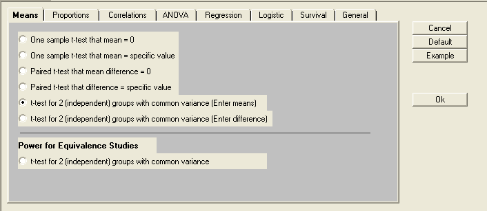
In Sample Power, it is fairly straightforward to perform power analysis for comparing means. Simply begin a new analysis and select ‘t-test for two independent groups with common variance [enter means]’.
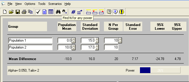
We can then specify the two means, the mean for Group 1 (diet A) and the mean for Group 2 (diet B). Since what really matters is the difference between the two values, we can enter a mean of zero for Group 1 and a mean of 10 for Group 2 so that the difference in means will be 10. Next, we specify the standard deviation for the first population and standard deviation for the second population. Note that upon entering a value for the second group, the following window will appear, to which ‘yes’ is the appropriate response.

From there, the default significance level (alpha level) is .05. For this example, we will set the power to be .8 by clicking the ‘Find N for any power’ button.

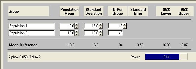
The calculation results indicate that we would need 42 subjects for diet A and another 42 subject for diet B in our sample in order to detect the specified difference with the given power. Now, let’s use another pair of means with the same difference. As we have discussed earlier, the results should be the same and we can see that they are.

A third way to the same result would be to begin a new project, designate ‘t-test for two independent groups with common variance [enter difference]’, and enter the difference between the means and the pooled standard deviation, which is the square root of the average of the two variances (squared standard deviations). In this case, it is sqrt((15^2 + 17^2)/2) ≈ 16.0. Despite the different types of inputs, we see an identical outcome.
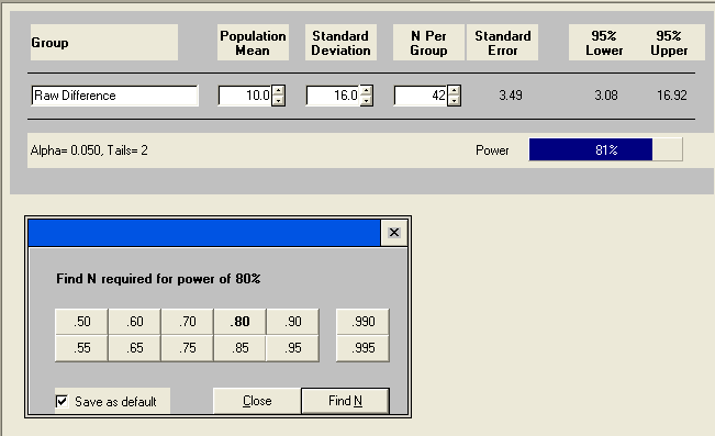
Now the dietician may feel that a total sample size of 82 subjects is beyond her budget. One way of reducing the sample size is to increase the Type I error rate, or the alpha level. Let’s say instead of using alpha level of .05 we will use .07, an adjustment accomplished by clicking the alpha value, then the blank value, and entering the new alpha value. As a result, our sample size decreases by 4 for each group as shown below.
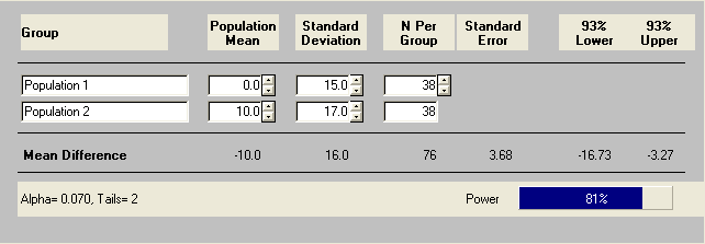
Now suppose the dietician can only collect data on 60 subjects with 30 in each group. What will the statistical power for her t-test be with respect to alpha level of .07?

What if she actually collected her data on 60 subjects but with 40 on diet A and 20 on diet B instead of equal sample sizes in the groups? Note that the N values will need to be unlinked, like the standard deviations were before.
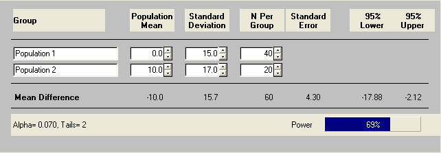
As you can see the power goes down from .72 to .69 even though the total number of subjects is the same. This is why we always say that a balanced design is more efficient.
Discussion
An important technical assumption is the normality assumption. If the distribution is skewed, then a small sample size may not have the power shown in the results because the power in the results is calculated using the normality assumption. We have seen that in order to compute the power or the sample size, we have to make a number of assumptions. These assumptions are used not only for the purpose of power calculations but in the actual t-test itself. So one important side benefit of performing power analysis is to help us to better understand our designs and our hypotheses.
We have seen in the power calculation process that what matters in the two-independent sample t-test is the difference in the means and the standard deviations for the two groups. This leads to the concept of effect size. In this case, the effect size will be the difference in means over the pooled standard deviation. The larger the effect size, the higher the power for a given sample size. Or the larger the effect size, the smaller the sample size needed to achieve a given level of power. Given this relationship, we can see that an accurate estimate of effect size is key to a good power analysis. However, it is not always an easy task to determine the effect size prior to collecting data. Good estimates of effect size often come from the existing literature or pilot studies.
For more information on power analysis, please visit our Introduction to Power Analysis seminar.
