SAS Code Fragments
Analyzing changes in trend over time
Create fake data set with given intercepts and slopes. Imagine a treatment and control group measured 5 times, then an intervention with 5 more observations. The intercepts and slopes are as shown in the data step.
NOTE: The analyses here simply focus on the meaning of the parameter estimates, and do NOT take into account correlations over time, covariance structures etc…
data hosp;
  do trt = 0 to 1;
    do int = 0 to 1;
      do year = 1 to 5;
	    if int = 0 and trt = 0 then y = 0+0*year ;
        if int = 1 and trt = 0 then y = 3+1*year ;
        if int = 0 and trt = 1 then y = 2+2*year ;
        if int = 1 and trt = 1 then y = 14+4*year ;
        year2 = year + 5*int;
		output;
	  end;
	end;
  end;
run;
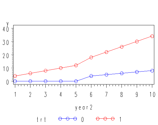
show plot of data
SYMBOL1 V=circle C=blue I=join;
SYMBOL2 V=circle C=red I=join;
proc gplot data=hosps;
  plot y*year2=trt;
run;

We use simple coding int as ints, trt as trts
data hosps;
  set hosp;
  ints = int - .5;
  trts = trt - .5;
run;
Show data
proc print data=hosps;
run;
Obs trt int year y year2 ints trts 1 0 0 1 0 1 -0.5 -0.5 2 0 0 2 0 2 -0.5 -0.5 3 0 0 3 0 3 -0.5 -0.5 4 0 0 4 0 4 -0.5 -0.5 5 0 0 5 0 5 -0.5 -0.5 6 0 1 1 4 6 0.5 -0.5 7 0 1 2 5 7 0.5 -0.5 8 0 1 3 6 8 0.5 -0.5 9 0 1 4 7 9 0.5 -0.5 10 0 1 5 8 10 0.5 -0.5 11 1 0 1 4 1 -0.5 0.5 12 1 0 2 6 2 -0.5 0.5 13 1 0 3 8 3 -0.5 0.5 14 1 0 4 10 4 -0.5 0.5 15 1 0 5 12 5 -0.5 0.5 16 1 1 1 18 6 0.5 0.5 17 1 1 2 22 7 0.5 0.5 18 1 1 3 26 8 0.5 0.5 19 1 1 4 30 9 0.5 0.5 20 1 1 5 34 10 0.5 0.5 |
Show slopes by int
b(int=0) is 1, b(int=1) is 2.5
proc sort data=hosps;
  by int;
run;

proc glm data=hosps;
  by int;
  model y = year / solution;
run;
<output abbreviated>
int=0
Standard Parameter Estimate Error t Value Pr > |t| Intercept 1.000000000 3.51781182 0.28 0.7834 year 1.000000000 1.06066017 0.94 0.3734 int=1
                                   Standard
Parameter         Estimate           Error    t Value    Pr > |t|
Intercept 8.500000000 8.47606925 1.00 0.3453 year 2.500000000 2.55563104 0.98 0.3566 |
show slopes by trt
b(trt=0) is .5, b(trt=1) is 3
proc sort data=hosps;
  by trt;
run;

proc glm data=hosps;
  by trt;
  model y = year / solution;
run;
trt=0 Standard Parameter Estimate Error t Value Pr > |t| Intercept 1.500000000 2.55563104 0.59 0.5734 year 0.500000000 0.77055175 0.65 0.5346 trt=1 Standard Parameter Estimate Error t Value Pr > |t| Intercept 8.000000000 7.55397246 1.06 0.3205 year 3.000000000 2.27760839 1.32 0.2243 |
run mixed analysis via simple coding
ints*trts*year is (4-1) – (2-0) = 1
ints*year is (2.5-1) = 1.5
trts*year is (3-.5) = 2.5
proc mixed data=hosps;
  model y = ints|trts|year / solution;
run;
<output abbreviated>
                              Standard
Effect            Estimate       Error      DF    t Value    Pr > |t|
Intercept 4.7500 0 12 Infty <.0001 ints 7.5000 0 12 Infty <.0001 trts 6.5000 0 12 Infty <.0001 ints*trts 9.0000 0 12 Infty <.0001 year 1.7500 0 12 Infty <.0001 ints*year 1.5000 0 12 Infty <.0001 trts*year 2.5000 0 12 Infty <.0001 ints*trts*year 1.0000 0 12 Infty <.0001 |
run mixed analysis via default (dummy) coding
after sas revises dummy codes (0=1, 1=0) slopes are
i=0 i=1
t=0 4 2
t=1 1 0
year = slope when i=0, t=0, = 4
y*i = change in slope for i, when t=0, 2-4 = -2
y*t = change in slope for t, when i=0, 1-4 = -3
i*t*y = (0-1) – (2-4) = -1 –2 = -1+2 = 1
proc mixed data=hosps;
  class int trt ;
  model y = int|trt|year / solution;
run;
<output abbreviated>
Solution for Fixed Effects
Intercept 14.0000 0 12 Infty <.0001 int 0 -12.0000 0 12 -Infty <.0001 int 1 0 . . . . trt 0 -11.0000 0 12 -Infty <.0001 trt 1 0 . . . . int*trt 0 0 9.0000 0 12 Infty <.0001 int*trt 0 1 0 . . . . int*trt 1 0 0 . . . . int*trt 1 1 0 . . . . year 4.0000 0 12 Infty <.0001 year*int 0 -2.0000 0 12 -Infty <.0001 year*int 1 0 . . . . year*trt 0 -3.0000 0 12 -Infty <.0001 year*trt 1 0 . . . . year*int*trt 0 0 1.0000 0 12 Infty <.0001 year*int*trt 0 1 0 . . . . year*int*trt 1 0 0 . . . . year*int*trt 1 1 0 . . . . |
