There are times when you want to do correspondence anlysis and the data have been collapsed into a summary with counts for each of the categories. For example, here is a dataset with the number of degrees given in 12 disciplines over eight different years.
discipline     1960       1965       1970       1971       1972       1973       1974       1975
    Agri        414        576        803        900        855        853        830        904
    Anth         69         82        217        240        260        324        381        385
     Bio       1245       1963       3360       3633       3580       3636       3473       3498
    Chem       1078       1444       2234       2204       2011       1849       1792       1762
   Earth        253        375        511        550        580        577        570        556
    Econ        341        538        826        791        863        907        833        867
     Eng        794       2073       3432       3495       3475       3338       3144       2959
    Math        291        685       1222       1236       1281       1222       1196       1149
     Oth        314        502       1079       1392       1500       1609       1531       1550
     Phy        530       1046       1655       1740       1635       1590        134       1293
   Psych        772        954       1888       2116       2262       2444       2587       2749
     Soc        162        239        504        583        638        599        645        680
We will begin by reading in the data.
data ca_summary;
 input disc $ v60 v65 v70 v71 v72 v73 v74 v75;
datalines;
     eng    794   2073   3432   3495   3475   3338   3144   2959
    math    291    685   1222   1236   1281   1222   1196   1149
     phy    530   1046   1655   1740   1635   1590    134   1293
    chem   1078   1444   2234   2204   2011   1849   1792   1762
    earth   253    375    511    550    580    577    570    556
     bio   1245   1963   3360   3633   3580   3636   3473   3498
    agri    414    576    803    900    855    853    830    904
   psych    772    954   1888   2116   2262   2444   2587   2749
   socio    162    239    504    583    638    599    645    680
    econ    341    538    826    791    863    907    833    867
  anthro     69     82    217    240    260    324    381    385
  others    314    502   1079   1392   1500   1609   1531   1550
;
run;
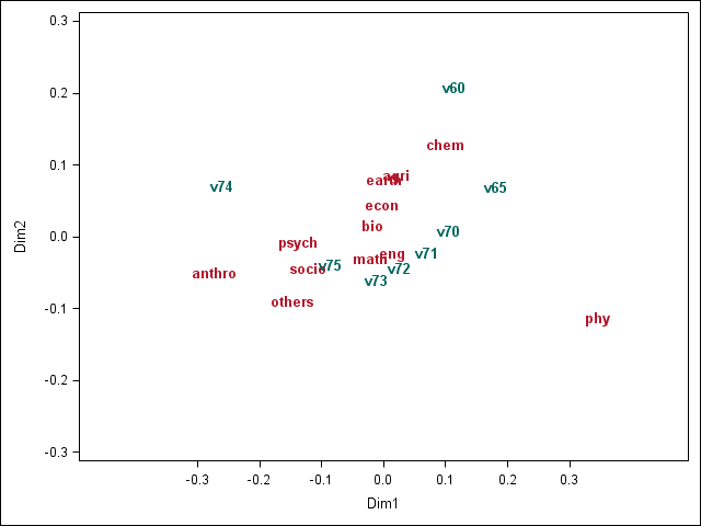
Now we are ready to run the correspondence analysis and plot the results.
proc corresp data=ca_summary out=coord short;
  var v60 v65 v70 v71 v72 v73 v74 v75;
  id disc;
run;

The CORRESP Procedure

                          Inertia and Chi-Square Decomposition

Singular    Principal       Chi-               Cumulative
  Value      Inertia     Square    Percent       Percent       14   28   42   56   70
                                                            ----+----+----+----+----+---
0.12662      0.01603    2031.34      68.55         68.55    ************************
0.06636      0.00440     557.91      18.83         87.38    *******
0.04960      0.00246     311.75      10.52         97.90    ****
0.01496      0.00022      28.36       0.96         98.86
0.01282      0.00016      20.81       0.70         99.56
0.00796      0.00006       8.04       0.27         99.83
0.00629      0.00004       5.01       0.17        100.00

  Total      0.02339    2963.21     100.00

Degrees of Freedom = 77

      Row Coordinates

              Dim1       Dim2

eng          0.0151    -0.0248
math        -0.0203    -0.0322
phy          0.3461    -0.1147
chem         0.1003     0.1269
earth        0.0002     0.0777
bio         -0.0182     0.0135
agri         0.0204     0.0835
psych       -0.1386    -0.0091
socio       -0.1218    -0.0459
econ        -0.0034     0.0432
anthro      -0.2726    -0.0515
others      -0.1475    -0.0918

     Column Coordinates

              Dim1       Dim2

v60          0.1142     0.2069
v65          0.1816     0.0676
v70          0.1048     0.0057
v71          0.0694    -0.0248
v72          0.0252    -0.0464
v73         -0.0114    -0.0631
v74         -0.2613     0.0695
v75         -0.0859    -0.0409

proc sgplot data = coord noautolegend;
 xaxis min = -.4 max = .4 values=(-.3 to .3 by .1) valueshint;
 yaxis min = -.3 max = .3;
 scatter x = dim1 y = dim2 /group = _type_ MARKERCHAR = disc
                            markercharattrs=(size=10 weight=bold);
run;