Making a 3-D Plot for a Logistic Regression | SAS Code Fragments

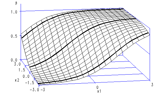
The example below shows how to generate a data set for a logistic regression
with two continuous predictors and plot the probability surface with respect to
the two predictors. It also shows how to use the annotate data set to add more
features to the plot.

data fig3_9;
  do i = 1 to 21;
     x1 = 6/20*(i -1) - 3;
    do j = 1 to 21;
     x2 = 6/20*(j-1) - 3;
     p = 1/(1+exp(-1 -1.1*x1 - .8*x2));
     output;
    end;
  end;
run;

/*creating the annotated data set*/
data x2_0a;
   length function  color $ 8 ;
   retain hsys xsys ysys zsys '1';
   retain line 1;
   retain size .75;
/*first extra thick line*/
     x = 0;
	 y = 5;
     z = 0;
	 function = 'move';
	 output;

	 do i = 2 to 21;
     x1 = 6/20*(i -1) - 3;
	 x= 5*(i-1);
     p = 1/(1+exp(-1 -1.1*x1 +.8*2.7));
	 y = 5;
	 z = 100*p;
     function = 'draw'; color='black';
	  output;
 end;

/*second extra thick line*/
     x = 0;
	 y = 50;
     z = 100/(1+exp(-1 + 1.1*3 )) ;
	 function = 'move';
	 output;

	 do i = 2 to 21;
     x1 = 6/20*(i -1) - 3;
	 x= 5*(i-1);
     p = 1/(1+exp(-1 -1.1*x1));
	 y = 50;
	 z = 100*p;
     function = 'draw'; color='black';
	 output;
 end;

/*third extra thick line*/
     x = 0;
	 y = 95;
     z = 100/(1+exp(-1 + 1.1*3 - .8*2.7)) ;
	 function = 'move';
	 output;

	 do i = 2 to 21;
     x1 = 6/20*(i -1) - 3;
	 x= 5*(i-1);
     p = 1/(1+exp(-1 -1.1*x1 - .8*2.7));
	 y = 95;
	 z = 100*p;
     function = 'draw'; color='black';
	 output;
 end;
run;

goptions  hsize=6 vsize=3.5;
proc g3d data = fig3_9 annotate=x2_0a;
  plot   x2*x1 = p / grid zticknum= 3  zmax = 1 zmin = 0 
                     rotate = 10 xticknum = 3 yticknum = 5 
                     caxis = blue ctop = black cbottom = gray;
run;
quit;