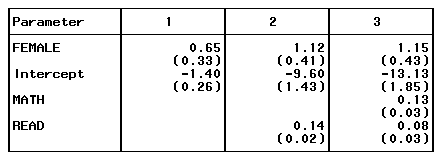
The following code creates a table of results for a series of logistic regressions. The resulting table will look like the one shown below. The coefficients for each variable is listed, each coefficient’s standard error is listed below it in parentheses.

As a first step, we need to define a format for the standard errors. Specifically, we need to tell SAS we want to set the number of decimal places displayed and put the value of the standard error in a set of parentheses ( "(" and ")" ). The picture statement tells SAS we want to create a format for printing numbers. The ‘ 9.99)’ tells SAS that we would like a number with up to two decimal places, and that the number should be followed by a ")". The (prefix='(‘) requests that the printed value be prefixed with "(". The final line instructs SAS that missing values should be shown as blank spaces.
proc format;
	picture stderrf (round)
     	low-high=' 9.99)' (prefix='(')
            .=' ';
run;
Next we use the output delivery system (ods) to capture the results from a series of regression models. The persist option allows ods to collect output from more than one run, otherwise output would be collected only for the first proc. Once ods is turned on we run a series of models using proc logistic. Below the regression models, we turn ods off (i.e. stop collecting information).
ods output ParameterEstimates (persist) = r;

proc logistic data = hsb2 desc;
  model hon = female;
run;
proc logistic data = hsb2 desc;
  model hon = female read;
run;
proc logistic data = hsb2 desc;
  model hon = female read math;
run;

ods output close;
Now the relevant coefficients etc. are stored in a dataset named r.
proc print data   = r;
run;
                                                                                          Prob
   Obs     _Proc_     _Run_    Variable     DF    Estimate      StdErr     WaldChiSq     ChiSq

    1     Logistic        1    Intercept     1     -1.4001      0.2632       28.3051    <.0001
    2     Logistic        1    FEMALE        1      0.6514      0.3337        3.8107    0.0509
    3     Logistic        1    Intercept     1     -9.6033      1.4264       45.3268    <.0001
    4     Logistic        1    FEMALE        1      1.1209      0.4081        7.5441    0.0060
    5     Logistic        1    READ          1      0.1444      0.0233       38.2785    <.0001
    6     Logistic        1    Intercept     1    -13.1266      1.8508       50.3034    <.0001
    7     Logistic        1    FEMALE        1      1.1547      0.4341        7.0761    0.0078
    8     Logistic        1    READ          1      0.0752      0.0276        7.4436    0.0064
    9     Logistic        1    MATH          1      0.1317      0.0325       16.4613    <.0001
Before we can display our output in a table, we will need to add a variable to our dataset that identifies which model each line in the dataset created by ods is associated with. The data step below creates a new dataset called r2 that includes a new variable modelnum which identifies the model each coefficient is associated with. Below that proc print is used to display the new dataset which contains the regression output as well as the variable modelnum. The retain statement tells SAS that the value of modelnum should start out the same as the value of modelnum in the case before it. The if statement changes the value of modelnum if the variable called variable is equal to "Intercept" which indicates that output from a new model begins with that case.
data r2;
  set r;
  retain modelnum 0;
  if variable="Intercept" then modelnum = modelnum + 1;
run;

proc print data   = r2;
run;

  Obs    _Proc_    _Run_   Variable    DF   Estimate     StdErr    WaldChiSq    ChiSq   modelnum

   1    Logistic       1   Intercept    1    -1.4001     0.2632      28.3051   <.0001       1
   2    Logistic       1   FEMALE       1     0.6514     0.3337       3.8107   0.0509       1
   3    Logistic       1   Intercept    1    -9.6033     1.4264      45.3268   <.0001       2
   4    Logistic       1   FEMALE       1     1.1209     0.4081       7.5441   0.0060       2
   5    Logistic       1   READ         1     0.1444     0.0233      38.2785   <.0001       2
   6    Logistic       1   Intercept    1   -13.1266     1.8508      50.3034   <.0001       3
   7    Logistic       1   FEMALE       1     1.1547     0.4341       7.0761   0.0078       3
   8    Logistic       1   READ         1     0.0752     0.0276       7.4436   0.0064       3
   9    Logistic       1   MATH         1     0.1317     0.0325      16.4613   <.0001       3
Now we can use proc tabulate to print our table. In the table statement, the first word variable indicates that the rows should be defined by the values of the variable of that name. That is, that there should be one row for each value of variable. The code estimate =' '*sum=' ' requests that the sum of the variable estimate be printed (since there is only one value of estimate for each combination of the variables variable and model, the sum is just the value itself). On the line below we do the same with the variable stderr except that *F=stderrf. applies the format we created above to the values. This takes care of defining what goes in the rows of our table. After the comma (",") we define the columns of our table. The variable name modelnum indicates that there should be one column in the table for each value of the variable modelnum. Throughout the command =' ' is used to set the label for the object it follows to blank.
proc tabulate data=r2 noseps;
  class modelnum variable;
  var estimate stderr;
  table variable=''*(estimate =' '*sum=' '
                     stderr=' '*sum=' '*F=stderrf.),
         modelnum=' '
          / box=[label="Parameter"] rts=15 row=float misstext=' ';
run;
See Also
