
Zero-inflated negative binomial regression is for modeling count variables with
excessive zeros and it is usually for over-dispersed count outcome variables.
Furthermore, theory suggests that the excess zeros are generated by a separate
process from the count values and that the excess zeros can be modeled
independently.
Please note: The
purpose of this page is to show how to use various data analysis commands. It
does not cover all aspects of the research process which researchers are
expected to do. In particular, it does not cover data cleaning and checking,
verification of assumptions, model diagnostics or potential follow-up analyses.
This page was updated using SAS 9.2.3.
Examples of Zero-inflated Negative Binomial Regression
Example 1. School administrators study the attendance behavior of high school
juniors at two schools. Predictors of the number of days of absence include
gender of the student and standardized test scores in math and language arts.
Example 2. The state wildlife biologists want to model how many fish are
being caught by fishermen at a state park. Visitors are asked how long they
stayed, how many people were in the group, were there children in the group and
how many fish were caught. Some visitors do not fish, but there is no data on
whether a person fished or not. Some visitors who did fish did not catch any
fish so there are excess zeros in the data because of the people that did not
fish.
Description of the Data
Let’s pursue Example 2 from above using the dataset
fish.sas7bdat.
We have data on 250 groups that went to a park. Each group was questioned
about how many fish they caught (count), how many children were in the
group (child), how many people were in the group (persons), and
whether or not they brought a camper to the park (camper).
In addition to predicting the number of fish caught, there is interest in predicting
the existence of excess zeros, i.e., the probability that a group caught zero
fish. We will use the variables child, persons, and camper
in our model.
Let’s look at the data.
proc means data = fish mean std min max var;
  var count child persons;
run;

The MEANS Procedure

Variable            Mean         Std Dev         Minimum         Maximum        Variance
----------------------------------------------------------------------------------------
count          3.2960000      11.6350281               0     149.0000000     135.3738795
child          0.6840000       0.8503153               0       3.0000000       0.7230361
persons        2.5280000       1.1127303       1.0000000       4.0000000       1.2381687
----------------------------------------------------------------------------------------
ods graphics / width=4in height=3in border=off; proc sgplot data = fish; histogram count /binwidth=1; run; ods graphics off;proc freq data = fish; tables child persons camper; run;
                                  Cumulative
child    Frequency     Percent     Frequency      Percent
----------------------------------------------------------
    0         132       52.80           132        52.80
    1          75       30.00           207        82.80
    2          33       13.20           240        96.00
    3          10        4.00           250       100.00


                                    Cumulative    Cumulative
persons    Frequency     Percent     Frequency      Percent
------------------------------------------------------------
      1          57       22.80            57        22.80
      2          70       28.00           127        50.80
      3          57       22.80           184        73.60
      4          66       26.40           250       100.00


                                   Cumulative    Cumulative
camper    Frequency     Percent     Frequency      Percent
-----------------------------------------------------------
     0         103       41.20           103        41.20
     1         147       58.80           250       100.00
proc means data = fish mean var n nway; class camper; var count; run;N camper Obs Mean Variance N ---------------------------------------------------------- 0 103 1.5242718 21.0557777 1031 147 4.5374150 212.4009878 147 ----------------------------------------------------------
We can see from the table of descriptive statistics above that the variance
of the outcome variable is quite large relative to the means. This might be an indication of over-dispersion.
Analysis methods you might consider
Before we show how you can analyze this with a zero-inflated negative binomial analysis, let’s
consider some other methods that you might use.
- OLS Regression – You could try to analyze these data using OLS regression. However, count
data are highly non-normal and are not well estimated by OLS regression. - Zero-inflated Poisson Regression – Zero-inflated Poisson regression does better when
the data are not over-dispersed, i.e., when variance is not much larger than the mean. - Ordinary Count Models – Poisson or negative binomial models might be more
appropriate if there are not excess zeros.
SAS zero-inflated negative binomial analysis using proc genmod
A zero-inflated model assumes that zero outcome is due to two different
processes. For instance, in the example of fishing presented here, the two
processes are that a subject has gone fishing vs. not gone fishing. If not gone fishing, the only
outcome possible is zero. If gone fishing, it is then a count
process. The two parts of the a zero-inflated model are a binary model, usually
a logit model to model which of the two processes the zero outcome is associated
with and a count model, in this case, a negative binomial model, to model the
count process. The expected count is expressed as a combination of the two
processes. Taking the example of fishing again, E(#of fish caught=k) = prob(not
gone fishing )*0 + prob(gone fishing)*E(y=k|gone fishing).
Now let’s build up our model. We are going to use the variables child and camper to model the
count in the part of negative binomial model and the variable persons
in the logit part of the model. The SAS commands are shown below. We treat variable camper as a categorical variable by
including it in the class statement. This will also make the post
estimations easier. In this particular example, we also explicitly want to use
camper = 0 as the reference group. To this end, we sort the data in descending
order and use the order= option in proc genmod to force it
to take camper = 0 as the reference group.
proc sort data = fish;
  by descending camper;
run;
proc genmod data = fish order=data;
  class camper;
  model count = child camper /dist=zinb;
  zeromodel persons;
run;
The GENMOD Procedure Model Information Data Set WORK.FISH Distribution Zero Inflated Negative Binomial Link Function Log Dependent Variable count Number of Observations Read 250 Number of Observations Used 250 Class Level Information Class Levels Values camper 2 1 0 Criteria For Assessing Goodness Of Fit Criterion DF Value Value/DF Deviance 865.7818 Scaled Deviance 865.7818 Pearson Chi-Square 245 534.2944 2.1808 Scaled Pearson X2 245 534.2944 2.1808 Log Likelihood -432.8909 Full Log Likelihood -432.8909 AIC (smaller is better) 877.7818 AICC (smaller is better) 878.1275 BIC (smaller is better) 898.9106 Algorithm converged.Analysis Of Maximum Likelihood Parameter Estimates Standard Wald 95% Confidence Wald Parameter DF Estimate Error Limits Chi-Square Pr > ChiSq Intercept 1 1.3710 0.2561 0.8691 1.8730 28.66 <.0001 child 1 -1.5153 0.1956 -1.8986 -1.1319 60.02 <.0001 camper 1 1 0.8791 0.2693 0.3513 1.4068 10.66 0.0011 camper 0 0 0.0000 0.0000 0.0000 0.0000 . . Dispersion 1 2.6788 0.4713 1.8974 3.7818 NOTE: The negative binomial dispersion parameter was estimated by maximum likelihood. Analysis Of Maximum Likelihood Zero Inflation Parameter Estimates Standard Wald 95% Wald Parameter DF Estimate Error Confidence Limits Chi-Square Pr > ChiSq Intercept 1 1.6031 0.8365 -0.0364 3.2426 3.67 0.0553 persons 1 -1.6666 0.6793 -2.9979 -0.3352 6.02 0.0142
The output has a few components which are explained below.
- Model Information: General information about the data set, outcome variable, distribution and the number of observations used in the model.
- Class Level Information: For each categorical variable, the number of
levels and how the levels are coded. The last displayed level will be the
reference group in the model. In this example, it will be 0. - Criteria For Assessing Goodness Of Fit: These measures are usually used
for comparing models. - Analysis Of Maximum Likelihood Parameter Estimates: Negative binomial
part of the model, estimated using maximum likelihood. - Analysis Of Maximum Likelihood Zero Inflation Parameter Estimates:
Logistic regression part of the model, for estimating the probability of
being an excessive zero.
Looking through the results of regression parameters we see the following:
- The predictors child and camper in the part of the negative binomial regression model predicting number
of fish caught (count) are both significant predictors. - The predictor person in the part of the logit model predicting
excessive zeros is statistically significant. - For these data, the expected change in log(count)
for a one-unit increase in child is -1.515255. This amounts to
a 78% (1 – e-1.515255 = .78) decrease in the expected count for each
additional child in the party holding other variables constant. - Groups with campers (camper = 1) had an expected log(count)
0.879051 higher than groups without campers (camper = 0), i.e., the
expected count of fish for a camper is about 2.41 (e0.879051 =
2.41) times higher than for a non-camper. - The log odds of being an excessive zero would decrease by 1.67 for every
additional person in the group. In other words, the more people in the group
,the less likely that the zero would be due to not gone fishing. Put it
plainly, the larger the group the person was in, the more likely that the
person went fishing. - The estimate of the dispersion parameter is displayed with its
confidence interval. There seems enough indication of over dispersion,
meaning that negative binomial model might be more appropriate.
Now, let’s try to understand the model better by using some of the post
estimation commands. First off, we examine the
distribution of the predicted probability of being an excessive zero by the number of persons in the group. We can see that the larger
the group, the smaller the probability, meaning the more likely that the person
went fishing.
proc means data = outzinb nway mean;
  class persons;
  var p0;
run;
N persons Obs Mean ----------------------------------- 1 57 0.4841404 2 70 0.1505843 3 57 0.0324022 4 66 0.0062858 -----------------------------------
Since we have saved our model previous as m1 previously, we use proc plm to get the predicted
number of fish caught, comparing campers with non-campers given different number
of children. To get the predict counts we have used the option
ilink (for inverse link).
proc plm source = m1;
  lsmeans camper /at child=(0) ilink;
  lsmeans camper /at child=(1) ilink;
  lsmeans camper /at child=(2) ilink;
  lsmeans camper /at child=(3) ilink;
run;
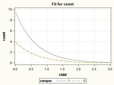
camper Least Squares Means Standard Standard Error of camper child persons Estimate Error z Value Pr > |z| Mean Mean 1 0.00 2.53 2.2501 0.2037 11.05 <.0001 9.4887 1.9326 0 0.00 2.53 1.3710 0.2561 5.35 <.0001 3.9395 1.0090 Standard Standard Error of camper child persons Estimate Error z Value Pr > |z| Mean Mean 1 1.00 2.53 0.7348 0.1932 3.80 0.0001 2.0852 0.4028 0 1.00 2.53 -0.1442 0.2342 -0.62 0.5381 0.8657 0.2028 Standard Standard Error of camper child persons Estimate Error z Value Pr > |z| Mean Mean 1 2.00 2.53 -0.7804 0.3311 -2.36 0.0184 0.4582 0.1517 0 2.00 2.53 -1.6595 0.3474 -4.78 <.0001 0.1902 0.06608 Standard Standard Error of camper child persons Estimate Error z Value Pr > |z| Mean Mean 1 3.00 2.53 -2.2957 0.5084 -4.52 <.0001 0.1007 0.05120 0 3.00 2.53 -3.1747 0.5128 -6.19 <.0001 0.04181 0.02144
Notice by default, SAS fixes the value of the predictor variable persons
at its mean value. Next, we can also ask proc plm to plot the fitted
values by camper variable.
ods graphics  / width=4in height=3in border=off;
proc plm source = m1;
  effectplot slicefit (sliceby= camper);
run;
ods graphics off;
Things to consider
Here are some issues that you may want to consider in the course of your
research analysis.
- Question about the over-dispersion parameter is in general a tricky one.
A large over-dispersion parameter could be due to a miss-specified model or
could be due to a real process with over-dispersion. Adding an
over-dispersion problem does not necessarily improve a miss-specified model. - The zinb model has two parts, a negative binomial count model and
the logit model for predicting excess zeros, so you might want to review
these Data Analysis Example pages,
Negative Binomial
Regression and
Logit Regression. - Since zinb has both a count model and a logit model, each of the
two models should have good predictors. The two models do not necessarily
need to use the same predictors. - Problems of perfect prediction, separation or partial separation can
occur in the logistic part of the zero-inflated model. - Count data often use exposure variable to indicate the number of times
the event could have happened. You can incorporate exposure into your model
by using the exposure() option. - It is not recommended that zero-inflated negative binomial models be
applied to small samples. What constitutes a small sample does not seem to
be clearly defined in the literature. - Pseudo-R-squared values differ from OLS R-squareds, please see
FAQ: What are pseudo R-squareds? for a discussion on this issue. - In times past, the Vuong test had been used to test whether a zero-inflated negative binomial model or a negative binomial model (without the zero-inflation) was a better fit for the data. However, this test is no longer considered valid. Please see The Misuse of The Vuong Test For Non-Nested Models to Test for Zero-Inflation by Paul Wilson for further information.
References
- Cameron, A. Colin and Trivedi, P.K. (2009) Microeconometrics using Stata.
College Station, TX: Stata Press. - Long, J. Scott, & Freese, Jeremy (2006). Regression Models for Categorical
Dependent Variables Using Stata (Second Edition). College Station, TX: Stata
Press. - Long, J. Scott (1997). Regression Models for Categorical and Limited
Dependent Variables. Thousand Oaks, CA: Sage Publications.
See also
- SAS Online Manual:
proc genmod - SAS macro program code:
Tests for comparing nested and nonnested models
modified on October 28, 2011