Applied Longitudinal Data Analysis: Modeling Change and Event Occurrenceby Judith D. Singer and John B. Willett Chapter 12: Extending the discrete-time hazard model

Table 12.2, page 413

Comparisons of alternate smooth polynomial representations for the main effect of time in a baseline discrete-time hazard model for the academic tenure data. First we create a constant variable called one (which is equal to one for all observations) as well as the higher order variables for time. We will make use of the ODS ability to select the output of fit statistics to a data set. To prepare us for the next example, we also make use of the out option of proc logistic to output the parameter estimates from a model to a corresponding data set.

data one;
  set 'c:\alda\tenure_pp';
  one = 1;
  time = period;
  time2 = period**2;
  time3 = period**3;
  time4 = period**4;
  time5 = period**5; 
run;
ods listing close;
 ods output fitstatistics (match_all=mnames persist=proc)=aic;
*general model;
proc logistic data=one out=general descending;
  model event = d1-d9 /noint;
run; 
*constant only model;
proc logistic data=one out=constant descending;
  model event = one /noint;
run; 
*linear model;
proc logistic data=one out=linear descending ;
  model event = one time /noint;
run; 
*quadratic model;
proc logistic data=one out=quadratic descending;
  model event =one time time2 /noint;
run;
*cubic model;
proc logistic data=one out=cubic descending ;
  model event = one time time2 time3 /noint;
run;
*fourth order model;
proc logistic data=one descending;
  model event =one time time2 time3 time4 /noint;
run;
*fifth order model;
proc logistic data=one descending;
  model event = one time time2 time3 time4 time5 /noint;
run;
ods output close;
ods listing;
*putting them together;
data allmodels;
  set &mnames;
  retain mnum;
  if criterion = "AIC" then mnum +1;
  if criterion ~="SC";
  drop withoutcovariates _proc_ _run_;
run;

proc transpose data = allmodels out=table12_2 (drop=_name_ _label_);
  by mnum;
  id criterion;
  var withcovariates;
run;
data table12_2a;
  set table12_2;
  retain gdev ;
  lagdev = lag(_2_log_l);
  if _n_ = 1 then gdev = _2_log_l;
  else do;
  if _n_ >2 then pdiff = lagdev -_2_log_l ;
  gdiff = _2_log_l - gdev;
  end;
  drop gdev lagdev;
 run;
 proc format ;
   value mname 1 = 'general'
               2 = 'constant'
               3 = 'linear'
	       4 = 'quadratic'
	       5 = 'cubic'
	       6 = 'fourth'
	       7 = 'fifth';
run;
proc print data = table12_2a noobs;
  format mnum mname.;
run;

mnum               AIC     _2_Log_L      pdiff     gdiff

general        849.204      831.204       .          .
constant      1039.565     1037.565       .       206.361
linear         871.462      867.462    170.103     36.258
quadratic      842.304      836.304     31.158      5.100
cubic          841.172      833.172      3.132      1.969
fourth         842.743      832.743      0.430      1.539
fifth          844.732      832.732      0.011      1.528

Figure 12.1, page 414

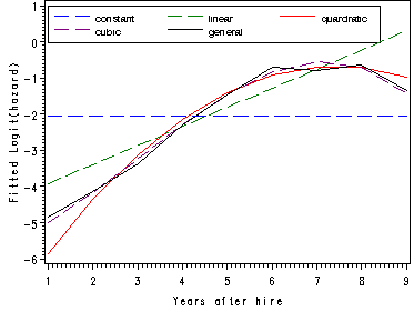
Comparing the fitted logit(hazard) curves from the models using different polynomial specification for time. In the previous proc logistic we have outputted data sets containing the estimates of the predictors in the model which will be used in computations to calculated the fitted logit(hazard) function for all the models. For the cubic and general model we will also calculate the fitted hazard and survival functions. The following is the data step to calculate the fitted logit(hazard) using the estimates that were outputted, in the data set constant, from the constant logistic model.

data constant(replace=yes);
  set constant;
  do year = 1 to 9;
    x0 = one ;
    output;
  end;
  keep year x0;
run;

The calculations needed to calculate the fitted logit(hazard) function using the estimates that were outputted, in the data set linear, from the linear logistic model.

data linear(replace=yes);
  set linear ;
  do year = 1 to 9;
    x1 = one + time*year  ;
    output;
  end;
  keep year x1;
run;

The calculations needed to calculate the fitted logit(hazard) function using the estimates that were outputted, in the data set quadratic, from the quadratic logistic model.

data quadratic(replace=yes);
  set quadratic;
  do year = 1 to 9;
    x2 = one + time*year + (time2)*(year**2) ;
    output;
  end;
  keep year x2;
run;

The calculations needed to calculate the fitted logit(hazard), the fitted hazard and the survival functions using the estimates that were outputted, in the data set cubic, from the cubic logistic model.

data cubic(replace=yes);
  set cubic;
  survivor3 = 1;
  do year = 1 to 9;
    x3 = one + time*year + (time2)*(year**2) + (time3)*(year**3);
    hazard3 = 1/(1 + exp(-x3));
    survivor3 = (1 - hazard3)*survivor3;
    output;
  end;
  keep year x3 survivor3 hazard3;
run;

The calculations needed to calculate the fitted logit(hazard), the fitted hazard and the survival functions using the estimates that were outputted, in the data set general, from the general logistic model.

data general(replace=yes);
  set general;
  array time[9] d1-d9;
  survivor9 = 1;
  do year = 1 to 9;
    x9 = time[year];
    hazard9 = 1/(1 + exp(-x9));
    survivor9 = (1 - hazard9)*survivor9;
    output;
  end;
  keep year x9 survivor9 hazard9;
run;

Merging all the datasets.

data all;
  merge constant linear quadratic cubic general;
  by year;
run;

The fitted logit(hazard) functions.

goptions reset=all;
symbol1 c=blue i=j l=21;
symbol2 c=green i=j l=21;
symbol3 c=red i=j l=1; *make bold;
symbol4  c=purple i=j l=21;
symbol5  c=black i=j l=1;
axis1 label=(a=90 'Fitted Logit(hazard)' );
axis2 label=('Years after hire');
legend1 label=none value=(height=1 font=swiss 'constant' 'linear' 'quardratic' 'cubic' 'general' )
        position=(top left inside) mode=share cborder=black down=2;
proc gplot data=all;
  plot (x0 x1 x2 x3 x9)*year/ overlay vaxis=axis1 haxis=axis2 legend=legend1;
run;
quit;

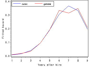
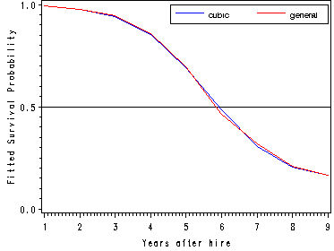
The fitted hazard and survival functions.

goptions reset=all;
symbol1 c=blue i=j;
symbol2 c=red i=j;
axis1 label=(a=90 'Fitted hazard') order=(0.0 to 0.4 by 0.1);
axis2 label=('Years after hire');
axis3 label=(a=90 'Fitted Survival Probability') order=(0.0 0.5 1.0);
legend1 label=none value=(height=1 font=swiss  'cubic' 'general' )
        position=(top left inside) mode=share cborder=black;
legend2 label=none value=(height=1 font=swiss  'cubic' 'general' )
        position=(top right inside) mode=share cborder=black;
proc gplot data=all;
  plot (hazard3 hazard9)*year/ overlay vaxis=axis1 haxis=axis2 legend=legend1;
  plot (survivor3 survivor9)*year / overlay vaxis=axis3 haxis=axis2 legend=legend2 vref=.5;
run;
quit;

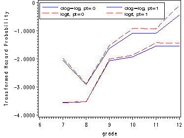
Figure 12.3, page423

In order to obtain the hazard probabilities for each level of pt using the different link functions: logit and clog-log, we need to run separate models for each level of pt for each link function. We start with fitting the model for pt=1 and using a clog-log link function. We use the ods output statement in order to capture the estimates for all the predictors in a separate data set, called cloglog0 without having to look at all other voluminous output from proc logistic.

ods listing close;
ods output  ParameterEstimates = cloglog0;
proc logistic data='c:\alda\firstsex_pp' descending ;
  where pt=0;
  model event = d7-d12 /noint link=cloglog;
run;
ods listing;
data cloglog0;
  set cloglog0;
  rename estimate = estc0;
  grade = substr(variable, 2, 2)+0;
  keep estimate grade;
run;
proc sort data=cloglog0;
 by grade;
run;

Here we do the same as in the previous code but for the model where pt=1 and the link is clog-log.

ods listing close;
ods output  ParameterEstimates = cloglog1;
proc logistic data='c:\alda\firstsex_pp' descending;
  where pt=1;
  model event = d7-d12 /noint link=cloglog;
run;
ods listing;
data cloglog1;
  set cloglog1;
  rename estimate = estc1;
  grade = substr(variable, 2, 2) +0;
  keep estimate grade;
run;
proc sort data=cloglog1;
 by grade;
run;

Here we do the same as in the previous code but for the model where pt=0 and the link is logit.

ods listing close;
ods output  ParameterEstimates = logit0;
proc logistic data='c:\alda\firstsex_pp' descending ;
  where pt=0;
  model event = d7-d12 /noint link=logit;
run;
ods listing;
data logit0;
  set logit0;
  rename estimate = estlog0;
  grade = substr(variable, 2, 2) +0;
  keep estimate grade;
run;
proc sort data=logit0;
 by grade;
run;

Here we do the same as in the previous code but for the model where pt=1 and the link is logit.

ods listing close;
ods output  ParameterEstimates = logit1;
proc logistic data='c:\alda\firstsex_pp' descending ;
  where pt=1;
  model event = d7-d12 /noint link=logit;
run;
ods listing;
data logit1;
  set logit1;
  rename estimate = estlog1;
  grade = substr(variable, 2, 2)+0;
  keep estimate grade;
run;
proc sort data=logit1;
 by grade;
run;

Merging all the data sets and graphing the hazard probabilities.


data graph;
  merge cloglog0 cloglog1 logit0 logit1;
  by grade;
run;
goptions reset=all;
symbol1 c=blue i=j;
symbol2 c=blue i=j;
symbol3 c=red i=j line=21;
symbol4 c=red i=j line=21;
axis1 label=(a=90 'Transformed Hazard Probability');
axis2 order=(6 to 12 by 1);
legend1 label=none position=(top left inside) mode=share cborder=black down=2
        value=(height=1 font=swiss  'clog-log, pt=0' 'clog-log, pt=1' 'logit, pt=0' 'logit, pt=1');
proc gplot data=graph;
  plot (estc0 estc1 estlog0 estlog1)*grade / overlay vaxis=axis1 haxis=axis2 legend=legend1;
run;
quit;

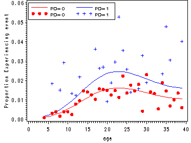
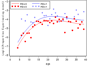
Figure 12.4, page 432

Proportion experience first depression onset by parental death.

proc means data='c:\alda\depression_pp' noprint;
  class pd period;
  var event;
  output out=sample mean(event)=percent;
run;
data sample;
set sample;
if 4<=period<=39 and 0<=pd<=1;
age = period;
parent = pd;
if percent = 0 then percent = .;
log_percent = log(percent/(1-percent) );
keep age parent percent log_percent;
run;

Fitting the logistic model with main effect of parental death.

proc logistic data='c:\alda\depression_pp' descending out=fitted noprint;
  model event = one age_18 age_18sq age_18cub pd/noint;
run;

Calculating.

data fitted(replace=yes);
  set fitted;
  do parent = 0 to 1;
    do age = 4 to 39;
      fitx = one + (age-18)*age_18 + ((age-18)**2)*age_18sq + ((age-18)**3)*(age_18cub)
             + pd*parent;
      fithazard = 1/(1 + exp(-fitx));
      output;
    end;
  end;
  keep parent age fitx fithazard;
run;

Merging the data sets.

data graph;
  merge sample fitted;
  by parent age;
  if parent=0 then do;
   sample0 = percent;
   x0 = fitx;
   hazard0 = fithazard;
   s0 = log_percent;
  end;
  if parent=1 then do;
   sample1 = percent;
   x1 = fitx;
   hazard1 = fithazard;
   s1 = log_percent;
  end;
  keep age sample0 x0 hazard0 s0 sample1 x1 hazard1 s1;
run;

Plots of the proportion experiencing the event and of the logit(proportion experiencing the event).

goptions reset=all;
symbol1 c=red i=j;
symbol2 c=blue i=j;
symbol3 v=dot c=red;
symbol4 v=plus c=blue;
axis1 label=(a=90 'Proportion Experiencing event');
axis2 label=(a=90 'Logit(Proportion Experiencing event)');
axis3 order=(0 to 40 by 5);
legend1 label=none value=(height=1 font=swiss 'PD=0' 'PD=1' 'PD=0' 'PD=1' )
        position=(top left inside) mode=share cborder=black down=2;
proc gplot data=graph;
title;
 plot (hazard0 hazard1 sample0 sample1 )* age / legend=legend1 overlay vaxis=axis1 haxis=axis3;
 plot (x0 x1 s0 s1)* age / legend=legend1 overlay vaxis=axis2 haxis=axis3;
run;
quit;

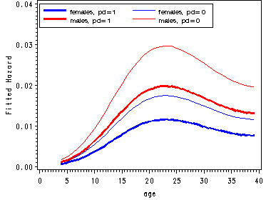
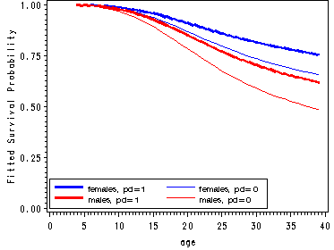
Figure 12.5, page 437

Fitted hazard functions for men and women split by pd.

proc logistic data='c:\alda\depression_pp' descending out=fitted;
  model event = one age_18 age_18sq age_18cub pd female/noint;
run;
data fitted(replace=yes);
set fitted;
do fem = 0 to 1;
do parent = 0 to 1;
survivor = 1;
do age = 4 to 39;
x = one + (age-18)*age_18 + ((age-18)**2)*age_18sq + ((age-18)**3)*(age_18cub)
+ pd*parent +female*fem;
hazard = 1/(1 + exp(-x));
survivor = (1-hazard)*survivor;
output;
end;
end;
end;
keep age parent fem hazard survivor;
run;
proc sort data=fitted;
by age fem parent;
run;
data estimates;
array haz[4] haz1-haz4;
array surv[4] surv1-surv4;
do i=1 to 4;
set fitted;
by age;
haz[i] = hazard;
surv[i] = survivor;
keep age haz1-haz4 surv1-surv4;
end;
run;
goptions reset=all;
symbol1 c=blue i=j width=2;
symbol2 c=blue i=j;
symbol3 c=red i=j width=2;
symbol4 c=red i=j;
axis1 order=(0 to 40 by 5);
axis2 label=(a=90 'Fitted Hazard') order=(0 to .04 by .01);
axis3 label=(a=90 'Fitted Survival Probability') order=(0 to 1 by .25);
legend1 label=none position=(top left inside) mode=share cborder=black down=2
value=(height=1 font=swiss 'females, pd=1' 'females, pd=0' 'males, pd=1' 'males, pd=0');
legend2 label=none position=(bottom left inside) mode=share cborder=black down=2
value=(height=1 font=swiss 'females, pd=1' 'females, pd=0' 'males, pd=1' 'males, pd=0');
proc gplot data=estimates;
plot (haz1 haz2 haz3 haz4)*age/ overlay legend=legend1 haxis=axis1 vaxis=axis2;
plot (surv1-surv4)*age / overlay legend=legend2 haxis=axis1 vaxis=axis3;
run;
quit;

Figure 12.6, page 445

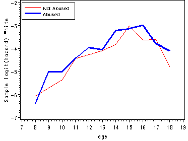
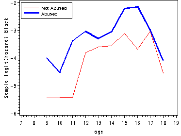
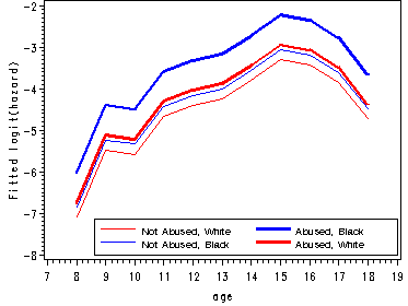
The first graph presents sample logit hazard functions computed separately for the two levels of the predictor abused. The second graph presents results for the white youths and the last graph presents the results for the black youths.

proc means data='c:\alda\firstarrest_pp' noprint;
  class period abused black;
  var event;
  output out=sample mean(event)=percent;
run;
data sample;
set sample;
if 8<=period<=18 and 0<=abused<=1 and 0<=black<=1;
age = period;
if percent = 0 then percent = .;
samp_logit=log(percent/(1-percent));
abuse=abused;
race=black;
keep age abuse race percent samp_logit;
run;

proc logistic data='c:\alda\firstarrest_pp' descending out=fitted;
model event = d8-d18 abused black ablack/noint;
run;

data fitted(replace=yes);
set fitted;
array timevar[11] d8-d18;
do abuse = 0 to 1;
do race = 0 to 1;
survivor = 1;
do age = 8 to 18;
fit_logit = timevar[age-7] + abuse*abused + race*black + abuse*race*ablack;
hazard = 1/(1 + exp(-fit_logit));
survivor = (1-hazard)*survivor;
output;
end;
end;
end;
keep age abuse race fit_logit hazard survivor;
run;

proc sort data=fitted;
by age race abuse;
run;
proc sort data=sample;
by age race abuse;
run;
data all;
merge fitted sample;
by age race abuse;
keep age race abuse samp_logit fit_logit;
run;
data estimates;
array samp[4] samp_logit1-samp_logit4;
array fit[4] fit_logit1-fit_logit4;
do i=1 to 4;
set all;
by age;
samp[i] = samp_logit;
fit[i] = fit_logit;
keep age samp_logit1-samp_logit4 fit_logit1-fit_logit4;
end;
run;
goptions reset=all;
symbol1 c=red i=j;
symbol2 c=blue i=j width=2;
symbol3 c=blue i=j ;
symbol4 c=red i=j width=2;
axis1 order=(7 to 19 by 1);
axis2 label=(a=90 'Sample logit(hazard) White');
axis3 label=(a=90 'Sample logit(hazard) Black');
axis4 label=(a=90 'Fitted logit(hazard)') order=(-8 to -2 by 1);
legend1 label=none position=(top left inside) mode=share cborder=black down=2
value=(height=1 font=swiss 'Not Abused' 'Abused');
legend2 label=none position=(bottom right inside) mode=share cborder=black down=2
value=(height=1 font=swiss 'Not Abused, White' 'Abused, Black'
'Not Abused, Black' 'Abused, White' );
proc gplot data=estimates;
plot (samp_logit1 samp_logit2)*age / overlay vaxis=axis2 haxis=axis1 legend=legend1;
plot (samp_logit3 samp_logit4)*age / overlay vaxis=axis3 haxis=axis1 legend=legend1;
plot (fit_logit1 fit_logit4 fit_logit3 fit_logit2)*age / overlay vaxis=axis3 haxis=axis1 legend=legend2;
run;
quit;

Table 12.4, page 449

Fitting three different discrete time models each using a different strategy for representing the sib-size effect. Model A uses the main effect of linear nsibs.

proc logistic data='c:\alda\depression_pp' descending ;
  model event = one age_18 age_18sq age_18cub pd female nsibs/noint;
run;

Model Fit Statistics

Without With Criterion Covariates Covariates

AIC 51288.732 4138.286 SC 51288.732 4197.916 -2 Log L 51288.732 4124.286

Testing Global Null Hypothesis: BETA=0

Test Chi-Square DF Pr > ChiSq

Likelihood Ratio 47164.4469 7 <.0001 Score 35471.2667 7 <.0001 Wald 7255.1495 7 <.0001

Analysis of Maximum Likelihood Estimates

Standard Wald Parameter DF Estimate Error Chi-Square Pr > ChiSq

ONE 1 -4.3587 0.1216 1284.7714 <.0001 age_18 1 0.0611 0.0117 27.4159 <.0001 age_18sq 1 -0.00731 0.00122 35.6482 <.0001 age_18cub 1 0.000182 0.000079 5.2883 0.0215 PD 1 0.3726 0.1624 5.2652 0.0218 FEMALE 1 0.5587 0.1095 26.0439 <.0001 NSIBS 1 -0.0814 0.0223 13.3605 0.0003

Table 12.4 model B Model B uses the main effect of categorized nsibs.

proc logistic data='c:\alda\depression_pp' descending ;
  model event = one age_18 age_18sq age_18cub pd female
                sibs12 sibs34 sibs56 sibs78 sibs9plus/noint;
run;

Model Fit Statistics

Without With Criterion Covariates Covariates AIC 51288.732 4139.982 SC 51288.732 4233.687 -2 Log L 51288.732 4117.982

Analysis of Maximum Likelihood Estimates

Standard Wald Parameter DF Estimate Error Chi-Square Pr > ChiSq ONE 1 -4.5001 0.2067 474.0222 <.0001 age_18 1 0.0615 0.0117 27.7578 <.0001 age_18sq 1 -0.00729 0.00122 35.4712 <.0001 age_18cub 1 0.000181 0.000079 5.2697 0.0217 PD 1 0.3727 0.1625 5.2616 0.0218 FEMALE 1 0.5596 0.1095 26.1017 <.0001 SIBS12 1 0.0209 0.1976 0.0111 0.9160 SIBS34 1 0.0108 0.2100 0.0026 0.9591 SIBS56 1 -0.4942 0.2545 3.7698 0.0522 SIBS78 1 -0.7754 0.3437 5.0893 0.0241 SIBS9PLUS 1 -0.6585 0.3441 3.6631 0.0556

Table 12.4, model C Model C uses the main effect of bigfamily.


proc logistic data='c:\alda\depression_pp' descending ;
  model event = one age_18 age_18sq age_18cub pd female bigfamily/noint;
run;

Model Fit Statistics

Without With Criterion Covariates Covariates AIC 51288.732 4132.778 SC 51288.732 4192.409 -2 Log L 51288.732 4118.778

Analysis of Maximum Likelihood Estimates

Standard Wald Parameter DF Estimate Error Chi-Square Pr > ChiSq ONE 1 -4.4828 0.1087 1700.3629 <.0001 age_18 1 0.0614 0.0117 27.7226 <.0001 age_18sq 1 -0.00729 0.00122 35.4867 <.0001 age_18cub 1 0.000182 0.000079 5.2809 0.0216 PD 1 0.3710 0.1623 5.2265 0.0222 FEMALE 1 0.5581 0.1095 25.9854 <.0001 BIGFAMILY 1 -0.6108 0.1446 17.8472 <.0001

Figure 12.8, page 458

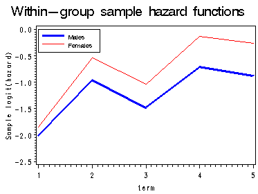
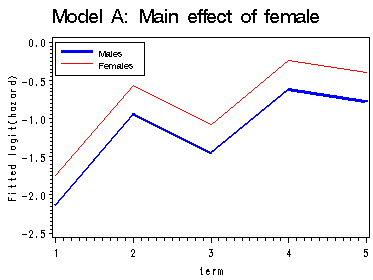
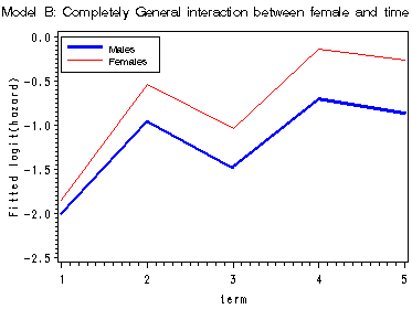
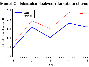
First graph presents the within-gender sample logit(hazard) functions, the fitted logit(hazard) for model A, B and C are presented in the last three graphs. Model A uses only the main effect of female; model B uses a completely general interaction between female and time; model C uses a linear interaction between female and time.

proc means data='c:\alda\mathdropout_pp' noprint;
  class female period;
  var event;
  output out=sample mean(event)=percent;
run;
data sample;
set sample;
if 1<=period<=5 and 0<=female<=1;
term = period;
fem = female;
if percent = 0 then percent = .;
sample_logit = log(percent/(1-percent));
keep term fem percent sample_logit;
run;
proc logistic data='c:\alda\mathdropout_pp' descending outest=A noprint;
model event = HS11 HS12 COLL1 COLL2 COLL3 FEMALE/noint;
run;

data a(replace=yes);
set a;
array time[5] hs11 hs12 coll1 coll2 coll3;
do fem = 0 to 1;
survivor_a = 1;
do term = 1 to 5;
x_a = time[term] + fem*female;
hazard_a = 1/(1 + exp(-x_a));
survivor_a = (1 - hazard_a)*survivor_a;
output;
end;
end;
keep term fem x_a survivor_a hazard_a;
run;
proc logistic data='c:\alda\mathdropout_pp' descending outest=B noprint;
model event = HS11 HS12 COLL1 COLL2 COLL3 FHS11 FHS12 FCOLL1 FCOLL2 FCOLL3/noint;
run;

data b(replace=yes);
set b;
array time[5] hs11 hs12 coll1 coll2 coll3;
array timeint[5] FHS11 FHS12 FCOLL1 FCOLL2 FCOLL3;
do fem = 0 to 1;
survivor_b = 1;
do term = 1 to 5;
x_b = time[term] + fem*timeint[term];
hazard_b = 1/(1 + exp(-x_b));
survivor_b = (1 - hazard_b)*survivor_b;
output;
end;
end;
keep term fem x_b survivor_b hazard_b;
run;
proc logistic data='c:\alda\mathdropout_pp' descending outest=C noprint;
model event = HS11 HS12 COLL1 COLL2 COLL3 female fltime/noint;
run;

data c(replace=yes);
set c;
array time[5] hs11 hs12 coll1 coll2 coll3;
do fem = 0 to 1;
survivor_c = 1;
do term = 1 to 5;
x_c = time[term] + fem*female + fem*fltime*(term-1);
hazard_c = 1/(1 + exp(-x_c));
survivor_c = (1 - hazard_c)*survivor_c;
output;
end;
end;
keep term fem x_c survivor_c hazard_c;
run;

data all;
merge sample a b c;
by fem term;
run;
proc print data=all;
by fem;
id term;
var sample_logit x_a x_b x_c;
run;

data final;
set all;
if fem = 0 then do;
sample0 = sample_logit;
a0 = x_a;
b0 = x_b;
c0 = x_c;
end;
if fem = 1 then do;
sample1 = sample_logit;
a1 = x_a;
b1 = x_b;
c1 = x_c;
end;
drop fem;
run;
goptions reset=all;
symbol1 c=blue i=j width=2;
symbol2 c=red i=j;
axis1 order=(-2.5 to 0 by .5) label=(a=90 'Sample logit(hazard)');
axis2 order=(-2.5 to 0 by .5) label=(a=90 'Fitted logit(hazard)');
legend label=none position=(top left inside) mode=share cborder=black down=2
value=(height=1 font=swiss 'Males' 'Females');
proc gplot data=final;
title 'Within-group sample hazard functions';
plot (sample0 sample1)*term /overlay legend=legend vaxis=axis1;
title 'Model A: Main effect of female';
plot (a0 a1 )*term / overlay legend=legend vaxis=axis2;
title 'Model B: Completely General interaction between female and time';
plot (b0 b1)*term / overlay legend=legend vaxis=axis2;
title 'Model C: Interaction between female and time';
plot (c0 c1)*term / overlay legend=legend vaxis=axis2;
run;
quit;
title;

Table 12.5, page 459

The parameter estimates, asymptotic standard deviations as well as deviance and AIC goodness of fit statistics. Model A: the main effects of female.

proc logistic data='c:\alda\mathdropout_pp' descending outest=A;
  model event = HS11 HS12 COLL1 COLL2 COLL3 FEMALE/noint;
run;

Model Fit Statistics

Without With Criterion Covariates Covariates AIC 13250.202 9816.310 SC 13250.202 9859.300 -2 Log L 13250.202 9804.310

Analysis of Maximum Likelihood Estimates

Parameter DF Estimate Error Chi-Square Pr > ChiSq HS11 1 -2.1308 0.0567 1410.3711 <.0001 HS12 1 -0.9425 0.0479 387.3380 <.0001 COLL1 1 -1.4495 0.0634 521.8728 <.0001 COLL2 1 -0.6176 0.0757 66.5471 <.0001 COLL3 1 -0.7716 0.1428 29.1962 <.0001 FEMALE 1 0.3786 0.0501 57.0104 <.0001

Table 12.5: Model B: completely general interaction of female and time.

proc logistic data='c:\alda\mathdropout_pp' descending outest=B;
  model event = HS11 HS12 COLL1 COLL2 COLL3 FHS11 FHS12 FCOLL1 FCOLL2 FCOLL3/noint;
run;

Model Fit Statistics

Without With Criterion Covariates Covariates AIC 13250.202 9816.270 SC 13250.202 9887.921 -2 Log L 13250.202 9796.270

Analysis of Maximum Likelihood Estimates

Standard Wald Parameter DF Estimate Error Chi-Square Pr > ChiSq HS11 1 -2.0077 0.0715 788.8764 <.0001 HS12 1 -0.9643 0.0585 271.2749 <.0001 COLL1 1 -1.4824 0.0847 306.2322 <.0001 COLL2 1 -0.7100 0.1007 49.6803 <.0001 COLL3 1 -0.8690 0.1908 20.7516 <.0001 FHS11 1 0.1568 0.0978 2.5716 0.1088 FHS12 1 0.4187 0.0792 27.9167 <.0001 FCOLL1 1 0.4407 0.1158 14.4811 0.0001 FCOLL2 1 0.5707 0.1445 15.5906 <.0001 FCOLL3 1 0.6008 0.2857 4.4208 0.0355

Table 12.5: Model C: linear interaction between female and time.

proc logistic data='c:\alda\mathdropout_pp' descending outest=C;
  model event = HS11 HS12 COLL1 COLL2 COLL3 female fltime/noint;
run;

Model Fit Statistics

Without With Criterion Covariates Covariates AIC 13250.202 9811.807 SC 13250.202 9861.962 -2 Log L 13250.202 9797.807

Analysis of Maximum Likelihood Estimates

Standard Wald Parameter DF Estimate Error Chi-Square Pr > ChiSq HS11 1 -2.0459 0.0646 1001.6547 <.0001 HS12 1 -0.9255 0.0482 368.5060 <.0001 COLL1 1 -1.4966 0.0665 506.5686 <.0001 COLL2 1 -0.7178 0.0861 69.5804 <.0001 COLL3 1 -0.9166 0.1557 34.6538 <.0001 FEMALE 1 0.2275 0.0774 8.6288 0.0033 FLTIME 1 0.1198 0.0470 6.4988 0.0108

Table 12.6, page 465

Deviance residuals from Model D of Table 3.3 for 8 boys in the grade at first intercourse data set.

proc logistic data='c:\alda\firstsex_pp' noprint descending;
  model event = d7-d12 PT PAS/noint;
  output out=resid resdev=resdev xbeta=xbeta p=p ;
run;
*creating the res variables for each time period--each period has a separate variable;
*creating the ssdev= sum(res**2) ;
data person;
  array resvar[6] res1-res6;
  do i=1 to 6 until (last.id);
    set resid;
    by id;
    resvar[i]=resdev;
  end;
  ssdev=uss(of res1-res6);
  censor = abs(event - 1);
  keep id ssdev event res1-res6 pt pas censor period grade;
run;
proc print data=person (rename=(period=time) ) noobs;
  where id=22 or id=112 or id=166 or id=89 or id=102 or id=87 or id=67 or id=212;
  var id pt pas time censor res1-res6 ssdev;
run;

ID PT PAS time censor res1 res2 22 1 -0.64965 12 0 -0.41173 -0.29444 67 1 2.27465 12 0 -0.61803 -0.44765 87 1 2.67790 7 0 1.81763 . 89 0 -0.07516 11 0 -0.32484 -0.23139 102 1 0.60493 8 0 -0.49134 2.36948 112 1 -0.66093 12 1 -0.41107 -0.29396 166 1 2.78141 11 0 -0.66145 -0.48068 212 0 -0.96179 12 1 -0.28570 -0.20322

res3 res4 res5 res6 ssdev -0.58404 -0.71765 -0.77477 1.41446 3.71332 -0.85591 -1.02943 -1.10073 1.04297 4.67406 . . . . 3.30378 -0.46446 -0.57518 1.86237 . 4.17403 . . . . 5.85584 -0.58314 -0.71659 -0.77366 -0.95629 2.62198 -0.91082 -1.09031 1.19140 . 4.10638 -0.40976 -0.50902 -0.55243 -0.69584 1.33930

Figure 12.9, page 467

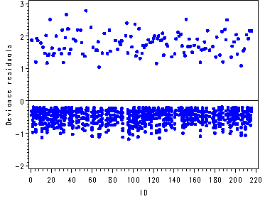
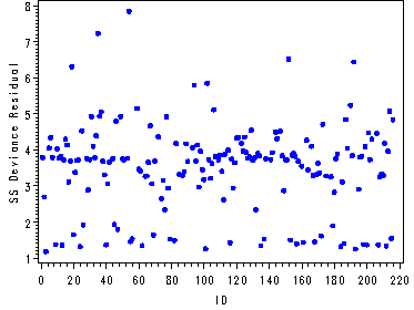
The first graph is an index plot of the deviance residuals for model D. The second graph is an index plot of the squared deviance residuals.

goptions reset=all;
symbol1 c=blue v=dot h=.7;
symbol2 c=blue v=dot h=.7;
symbol3 c=blue v=dot h=.7;
symbol4 c=blue v=dot h=.7;
symbol5 c=blue v=dot h=.7;
symbol6 c=blue v=dot h=.7;
axis1 order=(0 to 220 by 20);
axis2 label=(a=90 'Deviance residuals');
axis3 label=(a=90 'SS Deviance Residual');
proc gplot data=person;
  plot (res1-res6)*id / overlay haxis=axis1 vaxis=axis2 vref=0;
  plot ssdev*id / haxis=axis1 vaxis=axis3;
run;
quit;