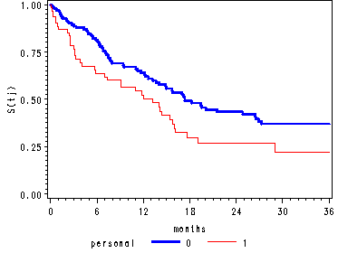
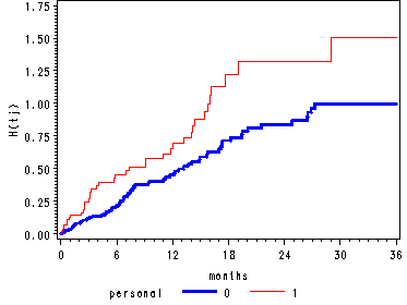
Figure 14.1, page 505
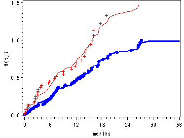
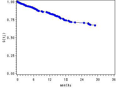
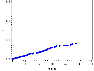
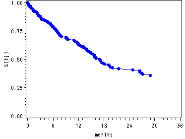
Two graphs: the Kaplan-Meier estimates of the survivor function and the negative log survivor estimates of the cumulative hazard function.
Note: the third graph of the kernel-smoothed estimates of the hazard function has not been included.
We output the Kaplan-Meier estimates to a data set called estimate using the outsurv option in the proc lifetest statement. We want add extra observations containing the values of the survival function for the greatest values of months for each level of personal, which has not been included since these values are censored. In order to accomplish this we first use proc means to obtain the greatest values for months where the estimates of the survival function is missing. Then we save these values as macros variables. The %put statement lets us see these macro variables in the log file.
proc lifetest data='c:aldarearrest' method=km outsurv=estimate noprint;
  time months*censor(1);
  strata personal;
run;
*finding the greates value for months where survival is not missing for each level of personal;
*saving these values as macros variables to be used in the next data step;
proc means data=estimate max;
  by personal;
  where survival ne .;
  var months;
run;

personal=0

The MEANS Procedure

Analysis Variable : months

     Maximum
------------
  27.2361396
------------

personal=1

Analysis Variable : months

     Maximum
------------
  28.9774127
------------

data _null_;
  set estimate;
  if personal = 0 and months ge 27 and survival ne . then call symput('surv0', survival);
  if personal = 1 and months ge 28 and survival ne . then call symput('surv1', survival);
run;
%put here are the two survival values: &surv0 and &surv1;
Adding the values of the survival function to the estimate data set.
*adding the last censored values for survival function and cumhaz function;
data two;
  set estimate;
  if _censor_ = 0 or (_censor_=1 and survival=.);
  interval+1;
  if months=36 and personal=0 then survival = &surv0;
  if months=36 and personal=1 then survival = &surv1;
  cumhaz = -log(survival);
  keep _censor_ interval months personal survival cumhaz;
run;
Finally, generating the two graphs.
goptions reset=all;
symbol1 i=stepjll c=blue width=2;
symbol2 i=stepjll c=red;
axis1 label=(a=90 'S(tj)') order=(0 to 1.0 by 0.25);
axis2 order=(0 to 36 by 6);
axis3 label=(a=90 'H(tj)') order=(0 to 1.75 by 0.25);
proc gplot data=two;
  plot survival*months = personal / vaxis=axis1 haxis=axis2;
  plot cumhaz*months  = personal /  vaxis=axis3 haxis=axis2;
run;
quit;
-----------------------------------------------------------------------------------------
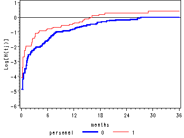
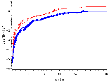
Figure 14.2, page 508
Figure 14.2–top panel
Graphing the log cumulative hazard function for the recidivism data.
First we create a data set, called null, containing the covariate pattern personal = 0. Then in proc phreg we can output the log of the cumulative hazard function for the covariate pattern in null by using the baseline statement with the loglogs option. Then we save the values of logh corresponding to the greatest value of months for which logh is non-missing as macro variables. These macros variables are used in the following data step where we create an extra observation at months=36 for each level of personal setting logh equal to the macro variables.
data null;
  input personal ;
  cards;
  0
;
run;
proc phreg data='c:aldarearrest' noprint;
  strata personal;
  model months*censor(1)= /ties=efron;
  baseline out=strata covariates=null logsurv=lsurv loglogs=logh /method=pl nomean;
run;
data _null_;
  set strata;
  if personal = 0 and months ge 27 then call symput('logh0', logh);
  if personal = 1 and months ge 28 then call symput('logh1', logh);
run;
%put here are the two survival values: &logh0 and &logh1; /*values displayed in the log file*/
data graph6_2;
  if _n_ = 1 then do;
    personal=0;
    months=36;
    logh=&logh0;
    output;
    personal=1;
    months=36;
    logh=&logh1;
  end;
  output;
  set strata;
run;
proc sort data=graph6_2;
  by months;
run;
goptions reset=all;
symbol1 i=stepjll c=blue width=2;
symbol2 i=stepjll c=red;
axis1 label=(a=90 'Log[H(tj)]') order=(-6 to 1.0 by 1);
axis2 order=(0 to 36 by 6);
proc gplot data=strata;
  plot logh*months=personal / overlay vaxis=axis1 haxis=axis2 vref=0;
run;
quit;
Figure 14.2–middle and lower panel
Log cumulative hazard functions and sample log cumulative hazard functions for each level of personal.
The first data step creates two data sets containing the variables months, h and logh, with one data set for each level of personal. These data sets are then sorted by the variable months.
data personal0 personal1;
  set strata;
  if personal=0 then do;
    th0 = -lsurv;
    tlogh0 = logh;
  end;
  if personal=0 then output personal0;
  if personal=1 then do;
    th1 = -lsurv;
	tlogh1 = logh;
  end;
  if personal=1 then output personal1;
run;
data personal0;
  set personal0;
  keep months th0 tlogh0;
run;
proc sort data=personal0;
  by months;
run;
data personal1;
  set personal1;
  keep months th1 tlogh1;
run;
proc sort data=personal1;
  by months;
run;
From proc phreg we output a data set called base using the baseline statement. This data set contains the survival function, the log of the survival function as well as the log of the cumulative hazard function for the covariate pattern where personal = 0. The data step is then used to create the hazard function for each level of personal as well as the log cumulative hazard function for personal = 1. We then save the values for both the hazard and the cumulative log hazard for each level of personal at the greatest value of months as macro variables. These are then used to create extra observations to the base data set. Then the data sets, personal0 and personal1, are merged with the base data set.
proc phreg data='c:aldarearrest' noprint;
  model months*censor(1)=personal /ties=efron;
  baseline out=base covariates=null survival=psurv0
           logsurv=lsurv0 loglogs=logh0 /method=pl nomean;
data base;
  set base;
  h0  = -lsurv0;
  h1 = h0*exp(0.47898);
  logh1 = logh0 + 0.47898;
  drop personal;
run;
data _null_;
  set base;
  if months ge 28 then call symput('h0', h0);
  if months ge 28 then call symput('h1', h1);
  if months ge 28 then call symput('logh0', logh0);
  if months ge 28 then call symput('logh1', logh1);
run;
%put here are the two survival values: &h0, &h1, &logh0 and &logh1;
*adding the last observations;
data base1;
  if _n_ = 1 then do;
    months=36;
    h0 = &h0;
    h1 = &h1;
    logh0 = &logh0;
    logh1 = &logh1;
  end;
  output;
  set base;
run;
proc sort data=base1;
  by months;
run;
data graph;
  merge base1 personal0 personal1;
  by months;
run;
goptions reset=all;
symbol1 i=j c=blue width=2;
symbol2 i=j c=red;
symbol3 c=blue v=dot i=none;
symbol4 c=red v=plus;
axis1 label=(a=90 'Log[H(tj)]') order=(-6 to 1.0 by 1);
axis2 order=(0 to 36 by 6);
axis3 label=(a=90 'H(tj)') order=(0 to 1.5 by .5);
proc gplot data=graph;
  plot (logh0 logh1 tlogh0 tlogh1)*months / overlay vaxis=axis1 haxis=axis2;
  plot (h0 h1 th0 th1)*months /  overlay vaxis=axis3 haxis=axis2;
run;
quit;
-----------------------------------------------------------------------------------------
Table 14.1, page 525
Results of fitting four Cox regression models to the recidivism data.
proc phreg data='c:aldarearrest';
  model months*censor(1)=personal/ties=efron;
run;

<output omitted>

         Model Fit Statistics

                 Without           With
Criterion     Covariates     Covariates
-2 LOG L         989.402        984.079
AIC              989.402        986.079
SBC              989.402        988.742

        Testing Global Null Hypothesis: BETA=0

Test                 Chi-Square       DF     Pr > ChiSq
Likelihood Ratio         5.3237        1         0.0210
Score                    5.6948        1         0.0170
Wald                     5.5964        1         0.0180

                     Analysis of Maximum Likelihood Estimates

                   Parameter      Standard                                  Hazard
Variable    DF      Estimate         Error    Chi-Square    Pr > ChiSq       Ratio
personal     1       0.47898       0.20247        5.5964        0.0180       1.614

proc phreg data='c:aldarearrest';
  model months*censor(1)=property/ties=efron;
run;

<output omitted>

         Model Fit Statistics

                 Without           With
Criterion     Covariates     Covariates
-2 LOG L         989.402        973.197
AIC              989.402        975.197
SBC              989.402        977.861


        Testing Global Null Hypothesis: BETA=0

Test                 Chi-Square       DF     Pr > ChiSq
Likelihood Ratio        16.2050        1         <.0001
Score                   13.1368        1         0.0003
Wald                    11.6970        1         0.0006

                     Analysis of Maximum Likelihood Estimates

                   Parameter      Standard                                  Hazard
Variable    DF      Estimate         Error    Chi-Square    Pr > ChiSq       Ratio
property     1       1.19459       0.34929       11.6970        0.0006       3.302


proc phreg data='c:aldarearrest';
  model months*censor(1)=cage/ties=efron;
run;

<output omitted>

         Model Fit Statistics

                 Without           With
Criterion     Covariates     Covariates
-2 LOG L         989.402        966.434
AIC              989.402        968.434
SBC              989.402        971.097

        Testing Global Null Hypothesis: BETA=0

Test                 Chi-Square       DF     Pr > ChiSq
Likelihood Ratio        22.9688        1         <.0001
Score                   19.1770        1         <.0001
Wald                    18.9997        1         <.0001

                     Analysis of Maximum Likelihood Estimates

                   Parameter      Standard                                  Hazard
Variable    DF      Estimate         Error    Chi-Square    Pr > ChiSq       Ratio
cage         1      -0.06812       0.01563       18.9997        <.0001       0.934

proc phreg data='c:aldarearrest';
  model months*censor(1)=personal property cage/ties=efron;
run;

<output omitted>

        Model Fit Statistics

                 Without           With
Criterion     Covariates     Covariates
-2 LOG L         989.402        950.442
AIC              989.402        956.442
SBC              989.402        964.432

        Testing Global Null Hypothesis: BETA=0

Test                 Chi-Square       DF     Pr > ChiSq
Likelihood Ratio        38.9602        3         <.0001
Score                   30.2968        3         <.0001
Wald                    29.0236        3         <.0001

                     Analysis of Maximum Likelihood Estimates

                   Parameter      Standard                                  Hazard
Variable    DF      Estimate         Error    Chi-Square    Pr > ChiSq       Ratio
personal     1       0.56914       0.20521        7.6920        0.0055       1.767
property     1       0.93579       0.35088        7.1128        0.0077       2.549
cage         1      -0.06671       0.01678       15.8094        <.0001       0.935
-----------------------------------------------------------------------------------------
Table 14.2, page 533
This table presents predictor values and risk scores for eight former inmates in the recidivism data.
proc phreg data='c:aldarearrest' noprint;
  id id;
  model months*censor(1)=personal property cage/ties=efron;
  output out=risk xbeta=xbeta;
run;
data risk;
  set risk;
  risk=exp(xbeta);
run;
proc print data=risk noobs;
  where id=22 or id=8 or id=187 or id=26 or id=5 or id=130 or id=106 or id=33;
  var id personal property cage xbeta risk months censor;
run;

 id    personal    property        cage      xbeta       risk      months    censor
  5        1           1        -7.1646     1.98290    7.26376     0.2957       0
  8        1           1        22.4507     0.00715    1.00718     0.6242       1
 22        0           0         0.2577    -0.01719    0.98295     1.7084       1
 26        0           1        -7.3015     1.42289    4.14911     2.3655       0
 33        1           0        27.0613    -1.23622    0.29048     2.7926       1
106        0           0        16.2030    -1.08096    0.33927    11.6961       0
130        0           1        22.3905    -0.55797    0.57237    15.9671       1
187        1           0        -7.2002     1.04949    2.85618    36.0000       1
-----------------------------------------------------------------------------------------
Figure 14.4, page 538
Figure 14.4--top and middle left panels
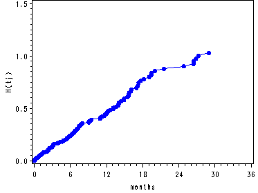
Graphing the survival function and cumulative hazard function for model D in Table 14.2 corresponding to the covariate pattern where all predictors in the model are equal to zero.
data null;
  input personal property cage;
  cards;
  0 0 0
;
run;
proc phreg data='c:aldarearrest' noprint;
  model months*censor(1)=personal property cage/ties=efron;
  baseline out=base0 covariates=null survival=survival
           logsurv=logs /method=pl nomean;
run;
data base0;
  set base0;
  haz  = -logs;
  drop logs personal property cage;
run;
goptions reset=all;
symbol v=dot c=blue i=j;
axis1 order=(0 to 1.0 by .25) label=(a=90 'S(tj)');
axis2 order=(0 to 1.0 by .25) label=(a=90 'H(tj)');
axis3 order=(0 to 36 by 6);
proc gplot data=base0;
  plot survival*months / vaxis=axis1 haxis=axis3;
  plot haz*months / vaxis=axis2 haxis=axis3;
run;
quit;
Figure 14.4--top and middle right panels
Graphing the survival function and cumulative hazard function for the model where all the predictors have been centered corresponding to the covariate pattern where all the centered predictors in the model are equal to zero. The proc sql is used to create the dataset containing the centered variables. The rest of the code is the same as for the preceding graphs.
proc sql;
  create table center as
  select *, personal - mean(personal) as cpersonal, property - mean(property) as cproperty
  from 'c:aldarearrest';
quit;
data null;
  input cpersonal cproperty cage;
  cards;
  0 0 0
;
run;
proc phreg data=center noprint;
  model months*censor(1)=cpersonal cproperty cage/ties=efron;
  baseline out=basem covariates=null survival=survival
           logsurv=logs /method=pl nomean;
run;
data basem;
  set basem;
  haz  = -logs;
  drop logs personal property cage;
run;
goptions reset=all;
symbol v=dot c=blue i=j;
axis1 order=(0 to 1.0 by .25) label=(a=90 'S(tj)');
axis2 order=(0 to 1.5 by .5) label=(a=90 'H(tj)');
axis3 order=(0 to 36 by 6);
proc gplot data=basem;
  plot survival*months / vaxis=axis1 haxis=axis3;
  plot haz*months / vaxis=axis2 haxis=axis3;
run;
quit;
-----------------------------------------------------------------------------------------
Figure 14.5, page 541
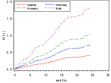
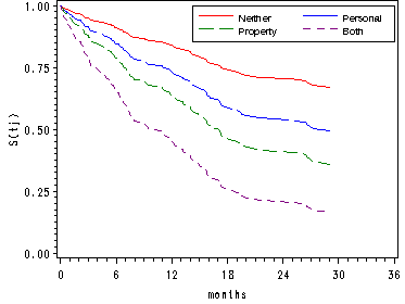
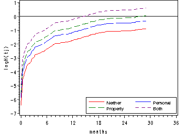
Using the data set base0 from Figure 14.4 which contains the baseline (all predictors equal to zero) for the survival function, the cumulative hazard and the log cumulative hazard functions. In the data step we create the cumulative hazard functions, the survival functions and the log cumulative hazard functions for the other covariate patterns.
data base1;
  set base0;
  cumhaz=haz;
  cumhazper = cumhaz*exp(0.5691);
  cumhazpro = cumhaz*exp(0.9358);
  cumhazboth = cumhaz*exp(1.5049);
  survper = exp(-cumhazper);
  survpro = exp(-cumhazpro);
  survboth = exp(-cumhazboth);
  logh=log(cumhaz);
  loghper = logh + 0.5691;
  loghpro = logh + 0.9358;
  loghboth = logh + 1.5049;
run;
goptions reset=all;
symbol1 c=red i=j;
symbol2 c=blue i=j l=23;
symbol3 c=green i=j l=21;
symbol4 c=purple i=j l=20;
axis1 order=(0 to 36 by 6);
axis2 order=(0 to 2 by .5) label=(a=90 'H(tj)');
axis3 order=(0 to 1 by .25) label=(a=90 'S(tj)');
axis4 order=(-7.0 to 1 by 1) label=(a=90 'logH(tj)');
legend1 label=none value=(height=1 font=swiss 'Neither' 'Personal' 'Property' 'Both' )
        position=(top left inside) mode=share cborder=black down=2;
legend2 label=none value=(height=1 font=swiss 'Neither' 'Personal' 'Property' 'Both' )
        position=(top right inside) mode=share cborder=black down=2;
legend3 label=none value=(height=1 font=swiss 'Neither' 'Personal' 'Property' 'Both' )
        position=(bottom right inside) mode=share cborder=black down=2;
proc gplot data=base1;
  plot (haz cumhazper cumhazpro cumhazboth)*months / overlay vaxis=axis2 haxis=axis1 legend=legend1;
  plot (survival survper survpro survboth)*months / overlay vaxis=axis3 haxis=axis1 legend=legend2;
  plot (logh loghper loghpro loghboth)*months / overlay vaxis=axis4 haxis=axis1 legend=legend3 vref=0;
run;
quit;

