Please note that the “early_int” data file (which is used in Chapter 3) is not included among the data files. This was done at the request of the researcher who contributed this data file to ensure the privacy of the participants in the study. Although the web page shows how to obtain the results with this data file, we regret that visitors do not have access to this file to replicate the results for themselves.
Note: This page is done using SAS 9.2 and we believe most if not all of the code will work in SAS 9.3 as well. This SAS code is based on code provided by Raymond R. Balise of Stanford University. We thank Raymond R. Balise for sharing his SAS 9.2 code with us.
Table 3.1, page 48
proc print data="c:\alda\earlyint_pp";
  where (id=68 or id=70 or id=71 or id=72 or id=902 or id=904 or id=906 or id=908);
  var id age cog program;
run;
Obs     ID    AGE    COG    PROGRAM
  1     68    1.0    103       1
  2     68    1.5    119       1
  3     68    2.0     96       1
  4     70    1.0    106       1
  5     70    1.5    107       1
  6     70    2.0     96       1
  7     71    1.0    112       1
  8     71    1.5     86       1
  9     71    2.0     73       1
 10     72    1.0    100       1
 11     72    1.5     93       1
 12     72    2.0     87       1
175    902    1.0    119       0
176    902    1.5     93       0
177    902    2.0     99       0
178    904    1.0    112       0
179    904    1.5     98       0
180    904    2.0     79       0
181    906    1.0     89       0
182    906    1.5     66       0
183    906    2.0     81       0
184    908    1.0    117       0
185    908    1.5     90       0
186    908    2.0     76       0
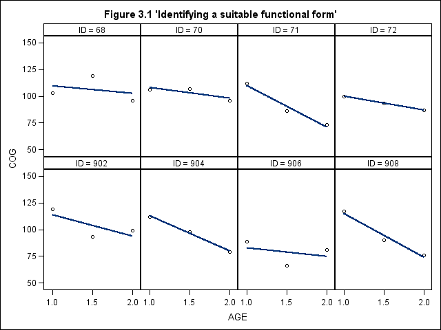
Figure 3.1, page 50
title "Figure 3.1 'Identifying a suitable functional form'";
proc sgpanel data = earlyint_pp noautolegend;
  where id in (68 70 71 72 902 904 906 908);
	panelby id / rows = 2 columns = 4;
	colaxis values = (1, 1.5, 2);
	rowaxis values = (50, 75, 100, 125, 150);
	reg x = age y = cog ;
run;
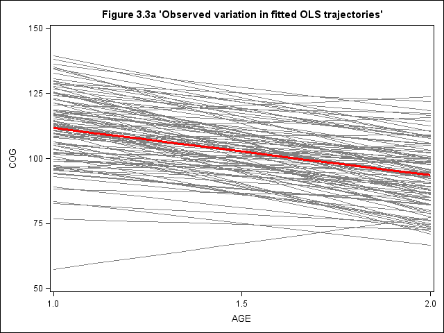
Figure 3.3, page 57
title "Figure 3.3a 'Observed variation in fitted OLS trajectories'";
proc sgplot data=earlyint_pp noautolegend ;
	xaxis values = (1, 1.5, 2);
	yaxis values = (50, 75, 100, 125, 150);
	reg x=age y=cog / group = id nomarkers LINEATTRS = (COLOR= gray PATTERN = 1 THICKNESS = 1) ;
	reg x=age y=cog/ nomarkers LINEATTRS = (COLOR= red PATTERN = 1 THICKNESS = 3) ;
run;
quit;
Figure 3.3 stem and leaf plots , page 57
data earlyint2;
  set "c:\alda\earlyint_pp";
  time = age-1;
run;

proc reg data=earlyint2 outest=ols rsquare noprint;
  model cog=time;
  by id;
run;

data ols;
  set ols;
  InitialStatus=Intercept;
  RateOfChange=Time;
  ResidualVariance=_rmse_**2;
  keep id initialstatus rateofchange residualvariance;
run;

* making step and leaf plots for bottom part of figure 3.3 ;
proc univariate data=ols plot;
  var initialstatus rateofchange residualvariance;
run;
The UNIVARIATE Procedure
Variable:  InitialStatus


   Stem Leaf                      #  Boxplot
     14 0                         1     |
     13 5568                      4     |
     13 00134                     5     |
     12 5556778999               10     |
     12 02233344                  8  +-----+
     11 55667777888889           14  |     |
     11 000111112222233334444    21  *--+--*
     10 55666688999              11  |     |
     10 0012222244               10  +-----+
      9 6666677799               10     |
      9 344                       3     |
      8 89                        2     |
      8 34                        2     |
      7 7                         1     |
      7
      6
      6
      5 7                         1     0
        ----+----+----+----+-
    Multiply Stem.Leaf by 10**+1
The UNIVARIATE Procedure
Variable:  RateOfChange


   Stem Leaf                     #  Boxplot
      2 0                        1     0
      1
      1 0                        1     |
      0 79                       2     |
      0 134                      3     |
     -0 4444332                  7     |
     -0 99998888777765          14  +-----+
     -1 4333322211000           13  |     |
     -1 99888877666655          14  *--+--*
     -2 44322211110000          14  |     |
     -2 9999877776655           13  +-----+
     -3 443322100000            12     |
     -3 987                      3     |
     -4 443111                   6     |
        ----+----+----+----+
    Multiply Stem.Leaf by 10**+1
The UNIVARIATE Procedure
Variable:  ResidualVariance


   Stem Leaf                                      #  Boxplot
     46 8                                         1     *
     44
     42
     40 00                                        2     *
     38
     36 8                                         1     *
     34
     32 3                                         1     0
     30
     28 4                                         1     0
     26 7                                         1     0
     24 1444                                      4     0
     22 8                                         1     |
     20                                                 |
     18 3                                         1     |
     16 00011                                     5     |
     14                                                 |
     12 21                                        2     |
     10 44433                                     5     |
      8 1118886666                               10  +-----+
      6 77744                                     5  |  +  |
      4 333844                                    6  |     |
      2 04444888833338888888                     20  *-----*
      0 0000111122233334444444466668111114447    37  +-----+
        ----+----+----+----+----+----+----+--
    Multiply Stem.Leaf by 10**+1
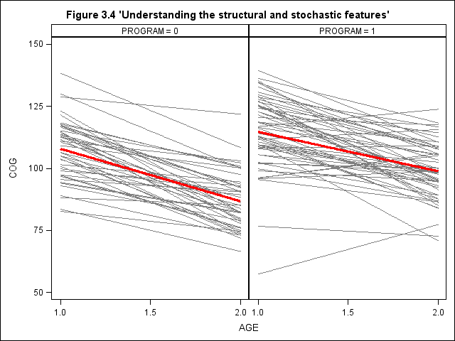
Figure 3.4, page 59
title "Figure 3.4 'Understanding the structural and stochastic features'";
proc sgpanel data = earlyint_pp noautolegend;
	panelby program / rows = 1 columns = 2;
	rowaxis min = 50 max = 150 values = (50, 75, 100, 125, 150);
	colaxis min = 1 max = 2 values = (1, 1.5, 2) VALUESHINT ;
	reg x = age y = cog /group = id nomarkers LINEATTRS = (COLOR= gray PATTERN = 1 THICKNESS = 1) ;
	reg x=age y=cog/ nomarkers LINEATTRS = (COLOR= red PATTERN = 1 THICKNESS = 3) ;
run;

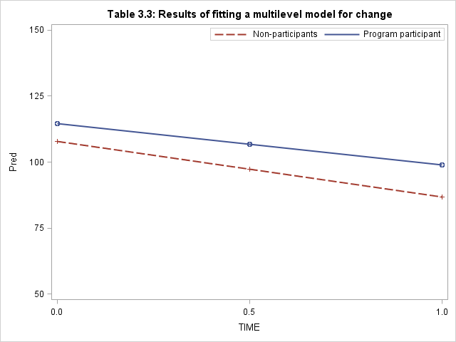
Table 3.3, page 69 and Figure 3.5 on page 70. Notice that in the proc mixed below, we made use of parms statement. This is because of the problem of non-positive definite G matrix when we didn’t have the initial values for variance-covariance matrix. The parms statement allows us to specify the lower and upper bound for each of the variance-covariance parameter and tell SAS to search for the optimal values on the grid defined by the number lists.
data earlyint2;
  set earlyint_pp;
  time = age-1;
run;
title1 "Table 3.3: Results of fitting a multilevel model for change";

ods exclude IterHistory ConvergenceStatus FitStatistics LRT;
proc mixed data=earlyint2 method=ml noclprint noinfo covtest;
  class id;
  model cog=time program time*program/solution notest outpm = work.predictedMean;
  random intercept time/type=un sub=id;
  parms  (120 to 126 by .5) (-37 to -35 by .5)
         (11 to 19 by 1) (72 to 74 by .5) / noiter noprofile;
run;
                  Covariance Parameter Estimates

                                    Standard         Z
Cov Parm     Subject    Estimate       Error     Value        Pr Z

UN(1,1)      ID           125.75     27.9642      4.50      <.0001
UN(2,1)      ID         -36.7181     23.3376     -1.57      0.1156
UN(2,2)      ID          11.0657     31.2760      0.35      0.3617
Residual                 74.4421     10.3768      7.17      <.0001
                    Solution for Fixed Effects

                            Standard
Effect          Estimate       Error      DF    t Value    Pr > |t|

Intercept         107.84      2.0428     101      52.79      <.0001
TIME            -21.1333      1.8853     101     -11.21      <.0001
PROGRAM           6.8547      2.7222     103       2.52      0.0133
TIME*PROGRAM      5.2713      2.5124     103       2.10      0.0383
proc format;
	value program
	1 = "Program participant"
	0 = "Non-participants";
run;

title "Figure 3.5 'Displaying the results of a fitted multilevel model'";
proc sgplot data=work.predictedMean;
	format program program.;
	xaxis values = (0, 0.5, 1);
	yaxis values = (50, 75, 100, 125, 150);
	reg x=age y=pred / group = program ;
	keylegend / location = inside position = topright;

run;


