Note: This page has been updated for SAS 9.3 and is based on SAS 9.2 code provided by Raymond R. Balise of Stanford University. We thank Raymond R. Balise for sharing his SAS 9.2 code with us.
Figure 4.1, page 77
title "Figure 4.1 'Identifying a suitable functional form'";
proc sgpanel data = alcohol1_pp (where = (id in (4, 14, 23, 32, 41, 56, 65, 82)))
     noautolegend  ;
  panelby id / columns = 4 rows = 2;
  colaxis values = (13, 14, 15, 16, 17) ;
  rowaxis min = 0 max = 4;
  reg x = age y = alcuse;
run;
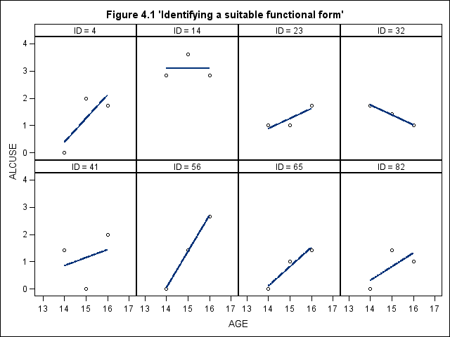
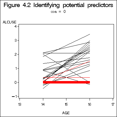
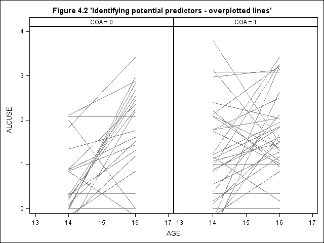
Figure 4.2, page 79. We will first present a simple-minded approach: no sub-sampling and no thickening the lines for coincident trajectories. The very much more complicated approach for sampling and adjusting the thickness of lines based on the number of coincidence of trajectories is presented afterwards.
title "Figure 4.2 'Identifying potential predictors - overplotted lines'";
proc sgpanel data = alcohol1_pp noautolegend ;
  panelby coa / columns = 2 rows = 1;
  colaxis values = (13 14, 15, 16, 17) ;
  rowaxis min = 0 max = 4 ;
  reg x = age y = alcuse / group = id nomarkers LINEATTRS = (COLOR= gray PATTERN = 1 THICKNESS = 1);
run;
proc sql;
  select mean(peer) into :mpeer
  from alcohol1_pp;
quit;
proc format;
  value peer
  low -< &mpeer = "Low PEER"
  &mpeer - high = "High PEER";
run;

title "Figure 4.2 'Identifying potential predictors - overplotted lines'";
proc sgpanel data = alcohol1_pp noautolegend;
  panelby peer / columns = 2 rows = 1 spacing = 5 novarname;
  format peer peer.;
  colaxis values = (13, 14, 15, 16, 17) ;
  rowaxis min = 0 max = 4 ;
  reg x = age y = alcuse / group = id nomarkers LINEATTRS = (COLOR= gray PATTERN = 1 THICKNESS = 1);
run;
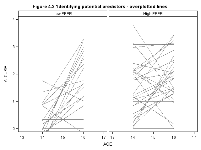
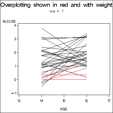
Now let us try to incorporate the idea of adjusting the thickness of the lines based on the number of coincidence of trajectories.
proc sort data = alcohol1_pp;
  by id coa;
run;
proc reg data = alcohol1_pp outest = parameters noprint;
  model alcuse = age_14;
  by id coa;
run;

proc sql;
  create table counts as
  select coa, intercept as b_int, age_14 as b_age, count(id) as weight
  from parameters
  group by coa, intercept, age_14
  order by weight;
quit;

data coa0 coa1 ;
  set counts;
  length function color $8;
  retain xsys ysys hsys '2';
  count = _N_;
  function = "move";
  size = weight/10;
  if weight > 1 then color = "red";
  else color = "black";
  x = 14; y = b_int;
  if coa = 0 then output coa0;
  else output coa1;
  function = "draw";
  x = 16; y = b_int + 2 * b_age;
  if coa = 0 then output coa0;
  else output coa1;
run;

goptions  reset = all ftext = swiss htitle = 5 htext = 3 gunit = pct
border cback = white hsize = 4in vsize = 4in;
filename outgraph 'c:\temp\mygraph1.gif';
goptions gsfname = outgraph dev = gif570;

axis1 order = (13 to 17 by 1) minor = none label=("AGE");
axis2 order = (-1 to 4 by 1)  minor = none label=("ALCUSE");
symbol1 v= none;
title "Figure 4.2 Identifying potential predictors";
title2 "coa = 0";
proc gplot data = coa0 (where = (coa = 0));
  plot y * x / anno = coa0  haxis = axis1 vaxis=axis2;
run;
quit;
filename outgraph 'c:temphttps://stats.idre.ucla.edu/wp-content/uploads/2016/02/mygraph2.gif';
goptions gsfname = outgraph dev = gif570;

title "Overplotting shown in red and with weight";
title2 "coa = 1";
proc gplot data = coa1 (where = (coa = 1));
  plot y * x / anno = coa1  haxis = axis1 vaxis=axis2;
run;
quit;
Table 4.1, pages 94-95
* Table 4.1 ;
title1 "Table 4.1: Alcohol use data (alcohol1_pp): Fitted multilevel models for change";
proc mixed data="c:\alda\alcohol1_pp" method=ml noclprint noinfo covtest;
  title2 "Model A";
  class id;
  model alcuse = /solution notest;
  random intercept/sub=id;

proc mixed data="c:\alda\alcohol1_pp" method=ml noclprint noinfo covtest;
  title2 "Model B";
  class id;
  model alcuse = age_14/solution notest;
  random intercept age_14/type=un sub=id;

proc mixed data="c:\alda\alcohol1_pp" method=ml noclprint noinfo covtest;
  title2 "Model C";
  class id;
  model alcuse = coa age_14 coa*age_14/solution notest;
  random intercept age_14/type=un sub=id;

proc mixed data="c:\alda\alcohol1_pp" method=ml noclprint noinfo covtest;
  title2 "Model D";
  class id;
  model alcuse = coa peer age_14 coa*age_14 peer*age_14 /solution notest;
  random intercept age_14/type=un sub=id;

proc mixed data="c:\alda\alcohol1_pp" method=ml noclprint noinfo covtest;
  title2 "Model E";
  class id;
  model alcuse = coa peer age_14 peer*age_14 /solution notest;
  random intercept age_14/type=un sub=id;

proc mixed data="c:\alda\alcohol1_pp" method=ml noclprint noinfo covtest;
  title2 "Model F";
  class id;
  model alcuse = coa cpeer age_14 cpeer*age_14 /solution notest;
  random intercept age_14/type=un sub=id;

proc mixed data="c:\alda\alcohol1_pp" method=ml noclprint noinfo covtest;
  title2 "Model G";
  class id;
  model alcuse = ccoa cpeer age_14 cpeer*age_14 /solution notest;
  random intercept age_14/type=un sub=id;
run;

Table 4.1: Alcohol use data (alcohol1_pp): Fitted multilevel models for change
Model A
                  Covariance Parameter Estimates

                                     Standard         Z
Cov Parm      Subject    Estimate       Error     Value        Pr Z
Intercept     ID           0.5639      0.1191      4.73      <.0001
Residual                   0.5617     0.06203      9.06      <.0001

           Fit Statistics
-2 Log Likelihood               670.2
AIC (smaller is better)         676.2
AICC (smaller is better)        676.3
BIC (smaller is better)         683.4

                   Solution for Fixed Effects

                         Standard
Effect       Estimate       Error      DF    t Value    Pr > |t|
Intercept      0.9220     0.09571      81       9.63      <.0001

Table 4.1: Alcohol use data (alcohol1_pp): Fitted multilevel models for change
Model B
                  Covariance Parameter Estimates

                                    Standard         Z
Cov Parm     Subject    Estimate       Error     Value        Pr Z
UN(1,1)      ID           0.6244      0.1481      4.22      <.0001
UN(2,1)      ID         -0.06844     0.07008     -0.98      0.3288
UN(2,2)      ID           0.1512     0.05647      2.68      0.0037
Residual                  0.3373     0.05268      6.40      <.0001

           Fit Statistics
-2 Log Likelihood               636.6
AIC (smaller is better)         648.6
AICC (smaller is better)        649.0
BIC (smaller is better)         663.1

  Null Model Likelihood Ratio Test
    DF    Chi-Square      Pr > ChiSq
     3         79.70          <.0001

                   Solution for Fixed Effects

                         Standard
Effect       Estimate       Error      DF    t Value    Pr > |t|
Intercept      0.6513      0.1051      81       6.20      <.0001
AGE_14         0.2707     0.06245      81       4.33      <.0001

Table 4.1: Alcohol use data (alcohol1_pp): Fitted multilevel models for change
Model C

                  Covariance Parameter Estimates

                                    Standard         Z
Cov Parm     Subject    Estimate       Error     Value        Pr Z
UN(1,1)      ID           0.4876      0.1278      3.81      <.0001
UN(2,1)      ID         -0.05934     0.06573     -0.90      0.3666
UN(2,2)      ID           0.1506     0.05639      2.67      0.0038
Residual                  0.3373     0.05268      6.40      <.0001

           Fit Statistics
-2 Log Likelihood               621.2
AIC (smaller is better)         637.2
AICC (smaller is better)        637.8
BIC (smaller is better)         656.5

  Null Model Likelihood Ratio Test

    DF    Chi-Square      Pr > ChiSq
     3         66.15          <.0001

                   Solution for Fixed Effects

                          Standard
Effect        Estimate       Error      DF    t Value    Pr > |t|
Intercept       0.3160      0.1307      80       2.42      0.0179
COA             0.7432      0.1946      82       3.82      0.0003
AGE_14          0.2930     0.08423      80       3.48      0.0008
COA*AGE_14    -0.04943      0.1254      82      -0.39      0.6944


Table 4.1: Alcohol use data (alcohol1_pp): Fitted multilevel models for change
Model D
                  Covariance Parameter Estimates

                                    Standard         Z
Cov Parm     Subject    Estimate       Error     Value        Pr Z
UN(1,1)      ID           0.2409     0.09259      2.60      0.0046
UN(2,1)      ID         -0.00612     0.05500     -0.11      0.9115
UN(2,2)      ID           0.1391     0.05481      2.54      0.0056
Residual                  0.3373     0.05268      6.40      <.0001

           Fit Statistics
-2 Log Likelihood               588.7
AIC (smaller is better)         608.7
AICC (smaller is better)        609.6
BIC (smaller is better)         632.8

  Null Model Likelihood Ratio Test

    DF    Chi-Square      Pr > ChiSq
     3         53.86          <.0001

                    Solution for Fixed Effects

                           Standard
Effect         Estimate       Error      DF    t Value    Pr > |t|
Intercept       -0.3165      0.1481      79      -2.14      0.0356
COA              0.5792      0.1625      82       3.56      0.0006
PEER             0.6943      0.1115      82       6.23      <.0001
AGE_14           0.4294      0.1137      79       3.78      0.0003
COA*AGE_14     -0.01403      0.1248      82      -0.11      0.9107
PEER*AGE_14     -0.1498     0.08564      82      -1.75      0.0840

Table 4.1: Alcohol use data (alcohol1_pp): Fitted multilevel models for change
Model E

                  Covariance Parameter Estimates

                                    Standard         Z
Cov Parm     Subject    Estimate       Error     Value        Pr Z
UN(1,1)      ID           0.2409     0.09259      2.60      0.0046
UN(2,1)      ID         -0.00614     0.05501     -0.11      0.9111
UN(2,2)      ID           0.1392     0.05481      2.54      0.0056
Residual                  0.3373     0.05268      6.40      <.0001

           Fit Statistics
-2 Log Likelihood               588.7
AIC (smaller is better)         606.7
AICC (smaller is better)        607.5
BIC (smaller is better)         628.4


  Null Model Likelihood Ratio Test

    DF    Chi-Square      Pr > ChiSq
     3         53.86          <.0001

                    Solution for Fixed Effects

                           Standard
Effect         Estimate       Error      DF    t Value    Pr > |t|
Intercept       -0.3138      0.1461      79      -2.15      0.0348
COA              0.5712      0.1462      82       3.91      0.0002
PEER             0.6952      0.1113      82       6.25      <.0001
AGE_14           0.4247      0.1056      80       4.02      0.0001
PEER*AGE_14     -0.1514     0.08451      82      -1.79      0.0770

Table 4.1: Alcohol use data (alcohol1_pp): Fitted multilevel models for change
Model F

                  Covariance Parameter Estimates

                                    Standard         Z
Cov Parm     Subject    Estimate       Error     Value        Pr Z
UN(1,1)      ID           0.2409     0.09259      2.60      0.0046
UN(2,1)      ID         -0.00614     0.05501     -0.11      0.9111
UN(2,2)      ID           0.1392     0.05481      2.54      0.0056
Residual                  0.3373     0.05268      6.40      <.0001

           Fit Statistics
-2 Log Likelihood               588.7
AIC (smaller is better)         606.7
AICC (smaller is better)        607.5
BIC (smaller is better)         628.4

  Null Model Likelihood Ratio Test

    DF    Chi-Square      Pr > ChiSq
     3         53.86          <.0001

                    Solution for Fixed Effects

                            Standard
Effect          Estimate       Error      DF    t Value    Pr > |t|
Intercept         0.3939      0.1035      79       3.80      0.0003
COA               0.5712      0.1462      82       3.91      0.0002
CPEER             0.6952      0.1113      82       6.25      <.0001
AGE_14            0.2706     0.06127      80       4.42      <.0001
CPEER*AGE_14     -0.1514     0.08451      82      -1.79      0.0770

Table 4.1: Alcohol use data (alcohol1_pp): Fitted multilevel models for change
Model G
      Covariance Parameter Estimates

                                    Standard         Z
Cov Parm     Subject    Estimate       Error     Value        Pr Z
UN(1,1)      ID           0.2409     0.09259      2.60      0.0046
UN(2,1)      ID         -0.00614     0.05501     -0.11      0.9111
UN(2,2)      ID           0.1392     0.05481      2.54      0.0056
Residual                  0.3373     0.05268      6.40      <.0001

           Fit Statistics
-2 Log Likelihood               588.7
AIC (smaller is better)         606.7
AICC (smaller is better)        607.5
BIC (smaller is better)         628.4

  Null Model Likelihood Ratio Test

    DF    Chi-Square      Pr > ChiSq
     3         53.86          <.0001

                    Solution for Fixed Effects

                            Standard
Effect          Estimate       Error      DF    t Value    Pr > |t|
Intercept         0.6515     0.07979      79       8.17      <.0001
CCOA              0.5712      0.1462      82       3.91      0.0002
CPEER             0.6952      0.1113      82       6.25      <.0001
AGE_14            0.2706     0.06127      80       4.42      <.0001
CPEER*AGE_14     -0.1514     0.08451      82      -1.79      0.0770
Table 4.1 (part 2), producing the output for pseudo R-squares which are described in Section 4.4.3 (page 102-104). We only show the code for Model D and the code can be applied for other models in this table.
1. An overall summary of total outcome variability explained
proc mixed data=alcohol1_pp  method=ml ;
  title2 "Model D";
  class id;
  model alcuse = coa peer age_14 coa*age_14 peer*age_14 /outpm=modeld;
  random intercept age_14/type=un sub=id;
run;
ods select fitstatistics;
proc reg data = modeld;
  model alcuse = pred;
run;
quit;
Root MSE 0.89686 R-Square 0.2912 Dependent Mean 0.92195 Adj R-Sq 0.2883 Coeff Var 97.278202. Pseudo R-squares computed from the variance components
*unconditional mean model;
ods output CovParms =m0;
proc mixed data=alcohol1_pp method=ml ;
  class id;
  unconditional: model alcuse = ;
  random intercept / sub=id;
run;

* unconditional growth model;
ods output covparms = m1;
proc mixed data=alcohol1_pp method=ml ;
  class id;
  growth: model alcuse = age_14 ;
  random intercept age_14/type=un sub=id;
run;

ods output covparms = m2;
*subsequent model;
proc mixed data=alcohol1_pp  method=ml ;
  title2 "Model D";
  class id;
  model alcuse = coa peer age_14 coa*age_14 peer*age_14;
  random intercept age_14/type=un sub=id;
run;

data _null_;
  set m0;
  if covparm="Residual" then call symput('sigma0', estimate);
run;
data _null_;
  set m1;
  if covparm="Residual" then call symput('sigma1', estimate);
  if covparm="UN(1,1)"  then call symput('xi01', estimate);
  if covparm="UN(2,2)"  then call symput('xi02', estimate);
run;
data _null_;
  set m2;
  if covparm="UN(1,1)" then call symput('xi1', estimate);
  if covparm="UN(2,2)" then call symput('xi2', estimate);
run;

data r2;
  r2_e = (&sigma0-&sigma1)/&sigma0;
  r2_0 = (&xi01 - &xi1)/&xi01;
  r2_1 = (&xi02 - &xi2)/&xi02;
run;
proc print data = r2;
run;
Obs r2_e r2_0 r2_1 1 0.39957 0.61415 0.079962
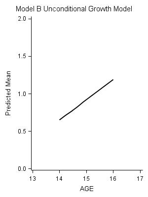
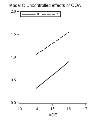
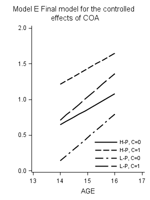
Figure 4.3 on page 99. The first two plots are based on the output data sets created by proc mixed using the outpm option after the model statement. The most right panel has to be created manually, since we have to create a new variable indicating the level of PEER.
ods graphics on /width=3in height=4in border=off;
proc mixed data=alcohol1_pp method=ml ;
  class id;
  model alcuse = age_14/outpm = mb;
  random intercept age_14/type=un sub=id;
run;


proc template;
	define style styles.alcohol;
		parent=styles.default;
		style GraphData1 from _self_/
		"LineStyle" = shortdash;
		style GraphData2 from _self_/
		"LineStyle" = mediumdash;
		style GraphData3 from _self_/
		"LineStyle" = mediumdashshortdash;
		style GraphData4 from _self_/
		"LineStyle" = mediumdashshortdash;
	end;
run;


ods html style = styles.alcohol;

title "Model B Unconditional Growth Model";
proc sgplot data=mb noautolegend;
	xaxis min = 13 max = 17;
	yaxis min = 0 max = 2;
	reg x=age y=pred /nomarkers  lineattrs=(color=black);
run;

proc mixed data=alcohol1_pp method=ml noclprint noinfo covtest;
  class id;
  model alcuse = coa age_14 coa*age_14/solution notest outpm = mc;
  random intercept age_14/type=un sub=id;
run;
title "Model C Uncontrolled effects of COA";
proc sgplot data=mc ;
  xaxis min = 13 max = 17;
  yaxis min = 0 max = 2 label=" ";
  reg x=age y=pred /group=coa   name="s1" nomarkers  lineattrs=(color=black) ;
  keylegend "s1"  / across= 2 location=inside ;
run;
data fig43r;
  do age = 14 to 16;
    do p = 0 to 1;
      do coa = 0 to 1;
	if p = 0 then peer = .655;
        if P = 1 then peer = 1.381;
        alcusehat = -.314 + .571*coa + .695*peer + .425*(age-14) + -.151*(age-14)*peer;
	if coa = 0 and p = 0 then coapeer = "L-P, C=0";
	if coa = 0 and p = 1 then coapeer = "H-P, C=0";
	if coa = 1 and p = 0 then coapeer = "L-P, C=1";
	if coa = 1 and p = 1 then coapeer = "H-P, C=1";
        output;
      end;
    end;
  end;
run;
Title "Model E Final model for the controlled effects of COA";


proc sgplot data=fig43r ;
  xaxis min = 13 max = 17 label="AGE";
  yaxis min = 0 max = 2 label =" ";
  reg x=age y=alcusehat / group = coapeer nomarkers  name="s1" lineattrs=(color=black);
  keylegend "s1"  /across=1 location=inside position=bottomright noborder;
run;
Table on the bottom of page 112.
proc sort data  = fig43r (where=(age<=15)) out=page112;
 by p coa age;
run;
data page112a;
   retain initial slope;
   set page112;
   lagp = lag(alcusehat);
   if age=14 then initial = alcusehat;
   if age = 15 then slope = alcusehat - lagp;
   drop lagp age;
   if age = 15;
run;
proc sort data = page112a;
 by p coa;

proc print data = page112a ;
 id coapeer;
 var initial slope;
run;
coapeer initial slope
Low Peer , COA=0    0.14123    0.32610
Low Peer , COA=1    0.71223    0.32610
High Peer, COA=0    0.64580    0.21647
High Peer, COA=1    1.21680    0.21647
Test of equation 4.18 on page 123 using model F.
proc mixed data=alcohol1_pp; method=ml;
  title2 "Model F";
  class id;
  model alcuse = coa cpeer age_14 cpeer*age_14 /solution chisq ;
  random intercept age_14/type=un sub=id;
  contrast 'Equation 4.18' intercept 1, age_14 1/ chisq ;
run;
The Mixed Procedure
                                   Contrasts
                  Num     Den
Label              DF      DF    Chi-Square    F Value      Pr > ChiSq    Pr > F
Equation 4.18       2      80         51.03      25.51          <.0001    <.0001
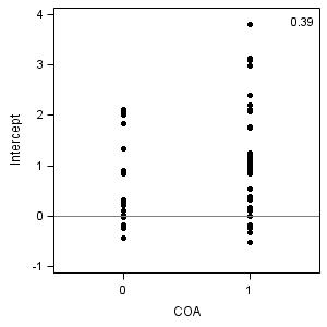
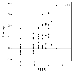
Figure 4.4 on page 130.
proc sort data = alcohol1_pp out=fig4_4;
 by id;
run;
proc reg data = fig4_4 outest=est plots=none noprint;
   by id;
  model alcuse = age_14;
run;
quit;
data fig4_4l;
  merge est(rename=(age_14=pred)) fig4_4;
  by id;
run;

ods output  PearsonCorr = corr;
proc corr data = fig4_4l nosimple noprob;
  var coa peer;
  with intercept pred;
run;
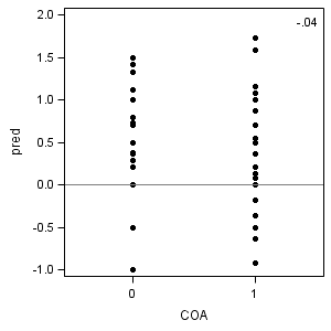
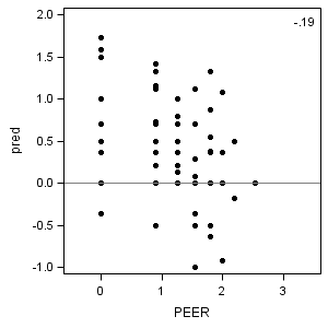
                    COA          PEER
Intercept       0.38867       0.57808
pred           -0.04349      -0.19404
data _null_;
  set corr;
  if _n_ = 1 then do;
    call symput('int_coa',  put(coa, 4.2));
    call symput('int_peer', put(peer, 4.2));
  end;
  if _n_ = 2 then do;
    call symput('pred_coa',  put(coa, 4.2));
    call symput('pred_peer', put(peer, 4.2));
  end;
run;
ods html style=journal2;
ods graphics on /width=3in height=3in border=off;
title;
proc sgplot data = fig4_4l;
 xaxis min = -.5 max = 1.5 values=(0,1) VALUESHINT;
 yaxis min = -1 max = 4 label="Intercept";
  format estimate 3.0;
  scatter x = coa  y = intercept  /markerattrs = (symbol=circlefilled);
  refline 0 /axis=y;
  inset  "&int_coa" /noborder position=topright;
run;
proc sgplot data = fig4_4l;
 xaxis min = -.5 max = 1.5 values=(0,1) VALUESHINT;
 yaxis min = -1 max = 2 label="pred";
  format estimate 3.0;
  scatter x = coa  y = pred  /markerattrs = (symbol=circlefilled);
  refline 0 /axis=y;
  inset  "&pred_coa" /noborder position=topright;
run;
proc sgplot data = fig4_4l;
 xaxis min = -.5 max = 3.5 values=(0,1,2,3) VALUESHINT;
 yaxis min = -1 max = 4 label="Intercept";
  format estimate 3.0;
  scatter x = peer  y = intercept  /markerattrs = (symbol=circlefilled);
  refline 0 /axis=y;
  inset  "&int_peer" /noborder position=topright;
run;
proc sgplot data = fig4_4l ;
 xaxis min = -.5 max = 3.5 values=(0,1,2,3) VALUESHINT;
 yaxis min = -1 max = 2 label="pred";
  format estimate 3.0;
  scatter x = peer  y = pred  /markerattrs = (symbol=circlefilled);
  refline 0 /axis=y;
  inset  "&pred_peer" /noborder position=topright;
run;
Figure 4.5 on page 131.
proc template;
   define style MyStyleDefault;
   parent=Styles.journal2;
   style Graph from Graph /OutputWidth = 4in OutputHeight=3in ;
   style GraphWalls from GraphWalls /FrameBorder = off;
   end;
run;
ods html style=MystyleDefault;
proc mixed data="c:aldaalcohol1_pp" covtest method=ml;
  title2 "Model F";
  class id;
  model alcuse = coa cpeer age_14 cpeer*age_14 / outp=fig4_5 solution chisq ;
  random intercept age_14/type=un sub=id solution;
  ods output SolutionR = fig4_5a;
run;
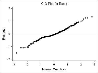
Part 1: Left upper one:
proc univariate data = fig4_5 noprint;
  var resid;
  qqplot /vref=0 ;
run;
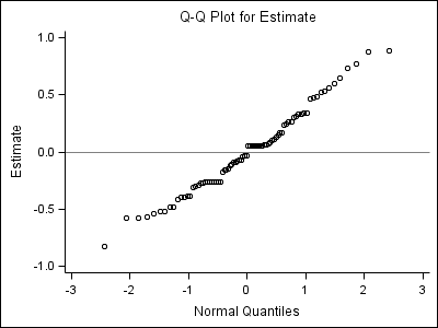
Part 2: Left middle one:
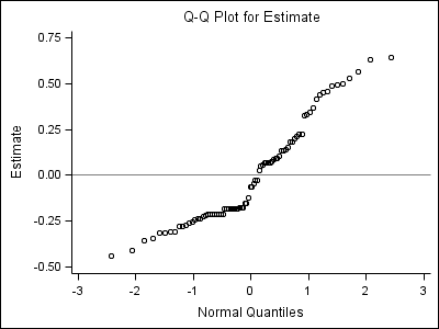
proc univariate data = fig4_5a noprint;
  where effect = "Intercept";
  var estimate;
  qqplot /vref=0 normal;
run;
Part 3: Left lower one:
proc univariate data = fig4_5a noprint;
  where effect = "AGE_14";
  var estimate;
  qqplot /vref=0 ;
run;
Part 4: Right upper one:
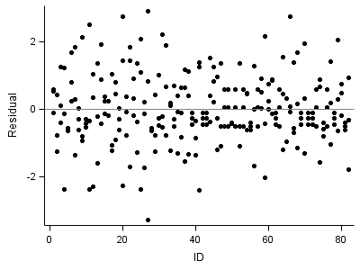
proc stdize data = fig4_5 out=fig4_5r;
  var resid;
run;
title;
proc sgplot data = fig4_5r;
  scatter x = id y = resid /markerattrs = (symbol=circlefilled);
  refline 0 /axis=y;
run;
quit;
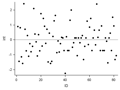
Part 5: Right middle one:
proc stdize data = fig4_5a out=fig4_5rm (rename=(estimate = int));
 where effect = "Intercept";
  var estimate;
run;
proc sgplot data = fig4_5rm;
  format int 3.0;
  scatter x = id y = int /markerattrs = (symbol=circlefilled);
  refline 0 /axis=y;
run;
Part 6: Right lower one:
proc stdize data = fig4_5a out=fig4_5rm (rename=(estimate=age));
 where effect = "AGE_14";
  var estimate;
run;
proc sgplot data = fig4_5rm;
  format age 3.0;
  scatter x = id y= age /markerattrs = (symbol=circlefilled);
  refline 0 /axis=y;
run;
quit;
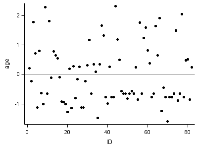
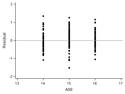
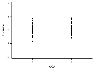
Figure 4.6 on page 133.
Part 1: Left upper plot:
proc sgplot data = fig4_5 ;
 xaxis min = 13 max = 17;
 yaxis min = -2 max = 2;
  scatter x = age y = resid /markerattrs = (symbol=circlefilled);
  refline 0 /axis=y;
run;
quit;
Part 2: Left middle plot:
proc sort data = fig4_a;
  by id;
proc sort data = alcohol1_pp;
  by id;
run;
data fig4_6int;
  merge fig4_5a (where=(effect="Intercept"))
        alcohol1_pp;
  by id;
run;
proc sgplot data = fig4_6int;
 xaxis min = -.5 max = 1.5 values=(0,1) VALUESHINT;
 yaxis min = -2 max = 2;
  format estimate 3.0;
  scatter x = coa y =  estimate /markerattrs = (symbol=circlefilled);
  refline 0 /axis=y;
run;
quit;
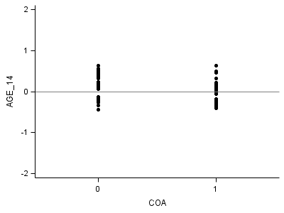
Part 3: Left lower plot:
data fig4_6age;
  merge fig4_5a (where=(effect="AGE_14"))
        alcohol1_pp;
  by id;
run;
proc sgplot data = fig4_6age;
 xaxis min = -.5 max = 1.5 values=(0,1) VALUESHINT;
 yaxis min = -2 max = 2 label="AGE_14";
  format estimate 3.0;
  scatter x = coa y =  estimate /markerattrs = (symbol=circlefilled);
  refline 0 /axis=y;
run;
quit;
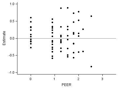
Part 4: Right middle plot:
proc sgplot data = fig4_6int;
 xaxis min = -.5 max = 3.5 values=(0,1, 2, 3) VALUESHINT;
 yaxis min = -1 max = 1 ;
  format estimate 3.0;
  scatter x = peer y =  estimate /markerattrs = (symbol=circlefilled);
  refline 0 /axis=y;
run;
quit;
Part 5: Right lower plot:
proc sgplot data = fig4_6age;
 xaxis min = -.5 max = 3.5 values=(0,1, 2, 3) VALUESHINT;
 yaxis min = -1 max = 1 ;
  format estimate 3.0;
  scatter x = peer y =  estimate /markerattrs = (symbol=circlefilled);
  refline 0 /axis=y;
run;
quit;
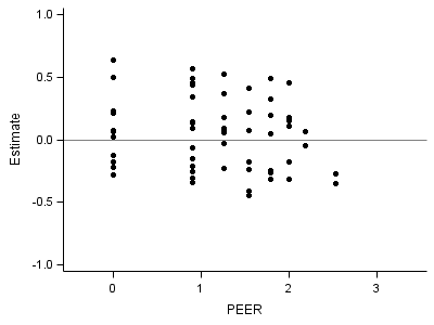
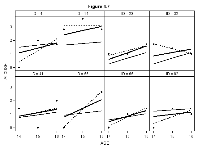
Figure 4.7 on page 136.
proc mixed data=alcohol1_pp covtest method=ml;
  title2 "Model F";
  class id;
  model alcuse = coa cpeer age_14 cpeer*age_14
		/outp=fig4_7p outpm = fig4_7pm  solution chisq ;
  random intercept age_14/type=un sub=id solution;
run;
proc sort data = fig4_7p;
  by id;
proc sort data = fig4_7pm;
  by id;
run;
data fig4_7;
  merge fig4_7p (rename = (pred=p)) fig4_7pm (rename=(pred=pm));
  by id;
  keep age id p pm alcuse;
  where id in (4,14,23,32,41,56,65,82);
run;
proc sort data = fig4_7;
  by id age;
run;
ods graphics on /reset = all;
title "Figure 4.7";
proc sgpanel data = fig4_7 noautolegend;
  panelby id /rows=2 columns=4;
  reg x = age y = alcuse / markerattrs= (symbol=circlefilled) LINEATTRS = (pattern = 2 COLOR= black);
  series x = age y = p / LINEATTRS = (pattern = 1 COLOR= black thickness=3);
  series x = age y = pm / LINEATTRS = (pattern = 1 COLOR= black thickness=2);
run;
