Note: This page is done using SAS 9.3 and is partly based on SAS code provided by Raymond R. Balise of Stanford University. We thank Raymond R. Balise for sharing his SAS 9.2 code with us.
Table 5.1 on page141.
title1 'Table 5.1 NLSY Reading study: 89 African American children';
proc print data='c:\alda\reading_pp';
  where id in (04,27,31,33,41,49,69,77,87);
  id id;
  var wave agegrp age piat;
run;

Table 5.1 NLSY Reading study: 89 African American children

ID    WAVE    AGEGRP      AGE      PIAT
 4      1       6.5      6.0000     18
 4      2       8.5      8.5000     31
 4      3      10.5     10.6667     50
27      1       6.5      6.2500     19
27      2       8.5      9.1667     36
27      3      10.5     10.9167     57
31      1       6.5      6.3333     18
31      2       8.5      8.8333     31
31      3      10.5     10.9167     51
33      1       6.5      6.3333     18
33      2       8.5      8.9167     34
33      3      10.5     10.7500     29
41      1       6.5      6.3333     18
41      2       8.5      8.7500     28
41      3      10.5     10.8333     36
49      1       6.5      6.5000     19
49      2       8.5      8.7500     32
49      3      10.5     10.6667     48
69      1       6.5      6.6667     26
69      2       8.5      9.1667     47
69      3      10.5     11.3333     45
77      1       6.5      6.8333     17
77      2       8.5      8.0833     19
77      3      10.5     10.0000     28
87      1       6.5      6.9167     22
87      2       8.5      9.4167     49
87      3      10.5     11.5000     64
Figure 5.1 on page 143.
data fig5_1;
  set "c:\alda\reading_pp";
  if id in (04,27,31,33,41,49,69,77,87);
run;
ods graphics /reset = all;
proc sgpanel data = fig5_1;
  panelby id /rows=3 columns=3 ;
  colaxis label="Age or age group";
  reg x = age y = piat / markerattrs = (symbol = circlefilled color = black)
          lineattrs = (color = black pattern = 2) legendlabel = "Age";;
  reg x = agegrp y = piat /markerattrs = (symbol = plus color = black)
          lineattrs = (color = black pattern = 1) legendlabel = "Age Group";;
run;
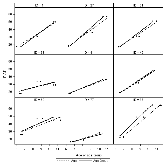
Table 5.2, page 145
data reading1;
  set 'c:\alda\reading_pp';
  cage=age-6.5;
  cagegrp=agegrp-6.5;
run;

proc mixed data=reading1 covtest noclprint noinfo noitprint method=ml;
  title1 'Table 5.2: Alternative representations for the main effect of TIME';
  title2 'Unconditional growth model';
  title3 'Using AGEGRP-6.5 as a temporal predictor';
  class id;
  model piat=cagegrp / solution notest ddfm=bw;
  random intercept cagegrp / subject=id type=un;
run;

proc mixed data=reading1 covtest noclprint noinfo noitprint method=ml;
  title3 'Using AGE-6.5 as a temporal predictor';
  class id;
  model piat=cage / solution notest ddfm=bw;
  random intercept cage / subject=id type=un;
run;
Table 5.2: Alternative representations for the main effect of TIME
Unconditional growth model
Using AGEGRP-6.5 as a temporal predictor
The Mixed Procedure
Covariance Parameter Estimates
                                    Standard         Z
Cov Parm     Subject    Estimate       Error     Value        Pr Z
UN(1,1)      ID          11.0459      6.0626      1.82      0.0342
UN(2,1)      ID           1.6467      2.0630      0.80      0.4248
UN(2,2)      ID           4.3975      1.2713      3.46      0.0003
Residual                 27.0431      4.0539      6.67      <.0001
Fit Statistics
-2 Log Likelihood              1819.9
AIC (smaller is better)        1831.9
AICC (smaller is better)       1832.3
BIC (smaller is better)        1846.9
Null Model Likelihood Ratio Test
DF Chi-Square Pr > ChiSq
3 86.92 <.0001
Solution for Fixed Effects
                         Standard
Effect       Estimate       Error      DF    t Value    Pr > |t|
Intercept     21.1629      0.6143      88      34.45      <.0001
cagegrp        5.0309      0.2956     177      17.02      <.0001
Table 5.2: Alternative representations for the main effect of TIME
Unconditional growth model
Using AGE-6.5 as a temporal predictor
The Mixed Procedure
Covariance Parameter Estimates
                                    Standard         Z
Cov Parm     Subject    Estimate       Error     Value        Pr Z
UN(1,1)      ID           5.1064      6.0299      0.85      0.1985
UN(2,1)      ID           2.3667      1.8022      1.31      0.1891
UN(2,2)      ID           3.3011      1.0145      3.25      0.0006
Residual                 27.4476      4.3720      6.28      <.0001
Fit Statistics
-2 Log Likelihood              1803.9
AIC (smaller is better)        1815.9
AICC (smaller is better)       1816.2
BIC (smaller is better)        1830.8
Null Model Likelihood Ratio Test
DF Chi-Square Pr > ChiSq
3 88.91 <.0001
Solution for Fixed Effects
                         Standard
Effect       Estimate       Error      DF    t Value    Pr > |t|
Intercept     21.0608      0.5593      88      37.65      <.0001
cage           4.5400      0.2606     177      17.42      <.0001
Table 5.3 on page 147.
title1 'Table 5.3: Excerpts from the person-period data set for the high school dropout study';
proc print data='c:\alda\wages_pp';
  where id in (206,332,1028);
  id id;
  var exper lnw black hgc uerate;
run;

Table 5.3: Excerpts from the person-period data set for the high school dropout

 ID     EXPER     LNW     BLACK    HGC    UERATE
 206    1.874    2.028      0       10     9.200
 206    2.814    2.297      0       10    11.000
 206    4.314    2.482      0       10     6.295
 332    0.125    1.630      0        8     7.100
 332    1.625    1.476      0        8     9.600
 332    2.413    1.804      0        8     7.200
 332    3.393    1.439      0        8     6.195
 332    4.470    1.748      0        8     5.595
 332    5.178    1.526      0        8     4.595
 332    6.082    2.044      0        8     4.295
 332    7.043    2.179      0        8     3.395
 332    8.197    2.186      0        8     4.395
 332    9.092    4.035      0        8     6.695
1028    0.004    0.872      1        8     9.300
1028    0.035    0.903      1        8     7.400
1028    0.515    1.389      1        8     7.300
1028    1.483    2.324      1        8     7.400
1028    2.141    1.484      1        8     6.295
1028    3.161    1.705      1        8     5.895
1028    4.103    2.343      1        8     6.900
Table 5.4 on page 149.
title1 'Table 5.4: Taxonomy of growth models to high school dropout wage data--Full ML';
proc mixed data='c:\alda\wages_pp' method=ml covtest noclprint noinfo;
  title2 'Model A: Unconditional growth model';
  class id;
  model lnw=exper / solution notest;
  random intercept exper / subject=id type=un;
run;

proc mixed data='c:\alda\wages_pp' method=ml covtest noclprint noinfo;
  title2 'Model B: Conditional growth model';
  title3 'effects of Black and HGC on both initial status and growth rate';
  class id;
  model lnw=exper hgc_9 hgc_9*exper black black*exper/solution notest;
  random intercept exper/subject=id type=un;
run;

proc mixed data='c:\alda\wages_pp' method=ml covtest noclprint noinfo;
  title2 'Model C: conditional growth model';
  title3 'HGC predicts initial status/BLACK predicts growth rate';
  class id;
  model lnw=exper hgc_9 black*exper /solution notest;
  random intercept exper/subject=id type=un;
run;

Table 5.4: Taxonomy of growth models to high school dropout wage data--Full ML
Model A: Unconditional growth model
The Mixed Procedure
Covariance Parameter Estimates
Standard Z Cov Parm Subject Estimate Error Value Pr Z
UN(1,1)      ID          0.05427    0.005001     10.85      <.0001
UN(2,1)      ID         -0.00291    0.000869     -3.35      0.0008
UN(2,2)      ID         0.001726    0.000220      7.84      <.0001
Residual                 0.09511    0.001944     48.92      <.0001
           Fit Statistics
-2 Log Likelihood              4921.4
AIC (smaller is better)        4933.4
AICC (smaller is better)       4933.4
BIC (smaller is better)        4962.1
  Null Model Likelihood Ratio Test
    DF    Chi-Square      Pr > ChiSq
     3       1580.05          <.0001
Solution for Fixed Effects
Standard Effect Estimate Error DF t Value Pr > |t| Intercept 1.7156 0.01080 887 158.90 <.0001 EXPER 0.04568 0.002341 850 19.51 <.0001
Table 5.4: Taxonomy of growth models to high school dropout wage data--Full ML
Model B: Conditional growth model
effects of Black and HGC on both initial status and growth rate
Covariance Parameter Estimates
Standard Z Cov Parm Subject Estimate Error Value Pr Z UN(1,1) ID 0.05175 0.004868 10.63 <.0001 UN(2,1) ID -0.00285 0.000844 -3.38 0.0007 UN(2,2) ID 0.001635 0.000214 7.65 <.0001 Residual 0.09520 0.001946 48.91 <.0001
Fit Statistics -2 Log Likelihood 4873.8 AIC (smaller is better) 4893.8 AICC (smaller is better) 4893.8 BIC (smaller is better) 4941.6
  Null Model Likelihood Ratio Test
    DF    Chi-Square      Pr > ChiSq
     3       1465.80          <.0001
Solution for Fixed Effects
Standard Effect Estimate Error DF t Value Pr > |t| Intercept 1.7171 0.01254 885 136.91 <.0001 EXPER 0.04934 0.002631 847 18.75 <.0001 HGC_9 0.03492 0.007881 4664 4.43 <.0001 EXPER*HGC_9 0.001280 0.001723 4664 0.74 0.4576 BLACK 0.01540 0.02393 4664 0.64 0.5200 EXPER*BLACK -0.01821 0.005498 4664 -3.31 0.0009
Table 5.4: Taxonomy of growth models to high school dropout wage data--Full ML
Model C: conditional growth model
HGC predicts initial status/BLACK predicts growth rate
Covariance Parameter Estimates
Standard Z Cov Parm Subject Estimate Error Value Pr Z UN(1,1) ID 0.05183 0.004873 10.64 <.0001 UN(2,1) ID -0.00288 0.000845 -3.41 0.0007 UN(2,2) ID 0.001646 0.000214 7.69 <.0001 Residual 0.09518 0.001945 48.92 <.0001
           Fit Statistics
-2 Log Likelihood              4874.7
AIC (smaller is better)        4890.7
AICC (smaller is better)       4890.7
BIC (smaller is better)        4929.0
  Null Model Likelihood Ratio Test
    DF    Chi-Square      Pr > ChiSq
     3       1474.50          <.0001
Solution for Fixed Effects
Standard Effect Estimate Error DF t Value Pr > |t| Intercept 1.7215 0.01070 886 160.93 <.0001 EXPER 0.04885 0.002513 849 19.44 <.0001 HGC_9 0.03836 0.006433 4663 5.96 <.0001 EXPER*BLACK -0.01612 0.004511 4663 -3.57 0.0004
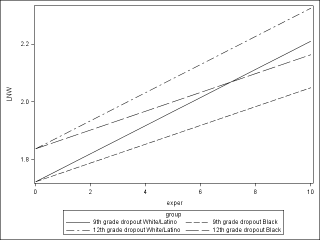
Figure 5.2 on page 150.
data fig5_2s;
  input exper hgc_9 black group $8-40;
datalines;
0  0 0  9th grade dropout White/Latino
10 0 0  9th grade dropout White/Latino
0  0 1  9th grade dropout Black
10 0 1  9th grade dropout Black
0  3 0  12th grade dropout White/Latino
10 3 0  12th grade dropout White/Latino
0  3 1  12th grade dropout Black
10 3 1  12th grade dropout Black
;
run;
data fig5_2sa;
   set fig5_2s;
   model1 = 1.7215 + 0.04885* exper + 0.03836*hgc_9 + -0.01612*exper*black;
run;
proc sgplot data= fig5_2sa;
   label model1 = "LNW";
   series x = exper y = model1 /group=group;
run;
Table 5.5 on page 154.
title1 'Table 5.5: Severely unbalanced data: Alternative approaches to model fitting';
title2 'Model C of Table 5.4';
proc mixed data='c:\alda\wages_small_pp' method=ml covtest noclprint noinfo;
  title3 'Approach A: Default method';
  class id;
  model lnw=exper hgc_9 black*exper /solution notest;
  random intercept exper/subject=id type=un;
run;

proc mixed data='c:\alda\wages_small_pp' method=ml covtest noclprint noinfo nobound;
  title3 'Approach B: Removing boundary constraints to allow negative variances';
  class id;
  model lnw=exper hgc_9 black*exper /solution notest;
  random intercept exper/subject=id type=un;
run;

proc mixed data='c:\alda\wages_small_pp' method=ml covtest noclprint noinfo;
  title3 'Approach C: Fixing rates of change';
  class id;
  model lnw=exper hgc_9 black*exper /solution notest;
  random intercept /subject=id type=un;
run;

Table 5.5: Severely unbalanced data: Alternative approaches to model fitting
Model C of Table 5.4
Approach A: Default method
The Mixed Procedure
Iteration History
Iteration Evaluations -2 Log Like Criterion
        0              1       307.58403963
        1              4       285.02372722       .
        2              1       283.93857489      0.00070544
        3              1       283.86897267      0.00000402
        4              1       283.86859250      0.00000000
Convergence criteria met.
Covariance Parameter Estimates
Standard Z Cov Parm Subject Estimate Error Value Pr Z UN(1,1) ID 0.08182 0.03344 2.45 0.0072 UN(2,1) ID 0.000627 0.006792 0.09 0.9264 UN(2,2) ID 7.54E-35 . . . Residual 0.1150 0.01475 7.80 <.0001
           Fit Statistics
-2 Log Likelihood               283.9
AIC (smaller is better)         297.9
AICC (smaller is better)        298.3
BIC (smaller is better)         317.6
  Null Model Likelihood Ratio Test
    DF    Chi-Square      Pr > ChiSq
     2         23.72          <.0001
Solution for Fixed Effects
Standard Effect Estimate Error DF t Value Pr > |t| Intercept 1.7373 0.04758 122 36.52 <.0001 EXPER 0.05159 0.02110 84 2.45 0.0165 HGC_9 0.04616 0.02447 47 1.89 0.0654 EXPER*BLACK -0.05963 0.03479 47 -1.71 0.0932
Table 5.5: Severely unbalanced data: Alternative approaches to model fitting
Model C of Table 5.4
Approach B: Removing boundary constraints to allow negative variances
The Mixed Procedure
Iteration History
Iteration Evaluations -2 Log Like Criterion
        0              1       307.58403963
        1              2       284.56884709      5.60876702
        2              1       284.25194563     35.06944214
        3              1       283.92785064    5019.4659324
        4              1       283.52412688    42196.186854
        5              1       282.74158921    497747.83733
        6              1       281.41649752    10711506.626
        7              1       279.61403087    437866210.81
        8              1       277.62479582     23604297296
        9              1       275.60074420    1.3418459E12
       10              1       273.57182583    7.6858612E13
       11              1       271.54226352    4.4071347E15
       12              1       269.51261608     2.527673E17
       13              1       267.48295914    1.4498933E19
       14              1       265.45328889    8.3175546E20
       15              1       263.42383149     4.771923E22
       16              1       261.39794939    2.7390031E24
       17              1       260.81549327    8.5330494E24
       18              1       260.24522738    2.6613477E25
       19              1       259.67583657    8.2813409E25
       20              0       259.67583657    8.2813409E25
       21              0       259.67583657    8.2813409E25
       22              0       259.67583657    8.2813409E25
       23              0       259.67583657    8.2813409E25
WARNING: Did not converge.
  Covariance Parameter Values
       At Last Iteration
Cov Parm Subject Estimate
UN(1,1)      ID          0.02665
UN(2,1)      ID          0.01954
UN(2,2)      ID         -0.00718
Residual                  0.1374
Table 5.5: Severely unbalanced data: Alternative approaches to model fitting
Model C of Table 5.4
Approach C: Fixing rates of change
The Mixed Procedure
Iteration History
Iteration Evaluations -2 Log Like Criterion 0 1 307.58403963 1 2 283.98842625 0.00110656 2 1 283.87813973 0.00000977 3 1 283.87721345 0.00000000
Convergence criteria met.
Covariance Parameter Estimates
Standard Z Cov Parm Subject Estimate Error Value Pr Z UN(1,1) ID 0.08424 0.02119 3.98 <.0001 Residual 0.1148 0.01455 7.89 <.0001
           Fit Statistics
-2 Log Likelihood               283.9
AIC (smaller is better)         295.9
AICC (smaller is better)        296.2
BIC (smaller is better)         312.8
  Null Model Likelihood Ratio Test
    DF    Chi-Square      Pr > ChiSq
     1         23.71          <.0001
Solution for Fixed Effects
Standard Effect Estimate Error DF t Value Pr > |t| Intercept 1.7373 0.04775 122 36.38 <.0001 EXPER 0.05178 0.02093 131 2.47 0.0147 HGC_9 0.04576 0.02450 131 1.87 0.0640 EXPER*BLACK -0.06007 0.03458 131 -1.74 0.0847
Table 5.6 on page 161.
title1 'Table 5.6: Excerpts from the person-period data set for the unemployment study';
proc print data='c:\alda\unemployment_pp';
  where id in (7589,55697,67641,65441,53782);
  id id;
  var months cesd unemp;
run;
Table 5.6: Excerpts from the person-period data set for the unemployment study
  ID      MONTHS    CESD    UNEMP
 7589     1.3142     36       1
 7589     5.0924     40       1
 7589    11.7947     39       1
53782     0.4271     22       1
53782     4.2382     15       0
53782    11.0719     21       1
55697     1.3470      7       1
55697     5.7823      4       1
65441     1.0842     27       1
65441     4.6982     15       1
65441    11.2690      7       0
67641     0.3285     32       1
67641     4.1068      9       0
67641    10.9405     10       0
Table 5.7 on page 163.
title1 'Table 5.7: Taxonomy of models of unemployment data';
proc mixed data='c:\alda\unemployment_pp' covtest noclprint noitprint noinfo method=ml;
  Title2 'Model A: Initial growth model';
  class id;
  model cesd=months / solution notest;
  random intercept months / subject=id type=un;
run;

proc mixed data='c:\alda\unemployment_pp' covtest noclprint noitprint noinfo method=ml;
  Title2 'Model B: Main effect of unemployment';
  class id;
  model cesd=months unemp / solution notest;
  random intercept months / subject=id type=un;
run;

proc mixed data='c:\alda\unemployment_pp' covtest noclprint noitprint noinfo method=ml;
  Title2 'Model C: Effect of unemployment on initial status and growth rate';
  class id;
  model cesd=months unemp unemp*months / solution notest;
  random intercept months / subject=id type=un;
run;

proc mixed data='c:\alda\unemployment_pp' covtest noclprint noitprint noinfo method=ml;
  Title2 'Model D: Allowing unemp to have both fix and random effects';
  class id;
  model cesd=unemp unemp*months / solution notest;
  random intercept unemp unemp*months / subject=id type=un;
run;

Table 5.7: Taxonomy of models of unemployment data
Model A: Initial growth model
The Mixed Procedure
Covariance Parameter Estimates
Standard Z Cov Parm Subject Estimate Error Value Pr Z UN(1,1) ID 86.8483 14.9631 5.80 <.0001 UN(2,1) ID -3.0572 1.3846 -2.21 0.0272 UN(2,2) ID 0.3550 0.1845 1.92 0.0272 Residual 68.8502 6.6027 10.43 <.0001
           Fit Statistics
-2 Log Likelihood              5133.1
AIC (smaller is better)        5145.1
AICC (smaller is better)       5145.3
BIC (smaller is better)        5166.4
  Null Model Likelihood Ratio Test
    DF    Chi-Square      Pr > ChiSq
     3        106.52          <.0001
Solution for Fixed Effects
Standard Effect Estimate Error DF t Value Pr > |t| Intercept 17.6694 0.7756 253 22.78 <.0001 MONTHS -0.4220 0.08298 226 -5.09 <.0001
Table 5.7: Taxonomy of models of unemployment data
Model B: Main effect of unemployment
The Mixed Procedure
Covariance Parameter Estimates
Standard Z Cov Parm Subject Estimate Error Value Pr Z UN(1,1) ID 93.5189 14.8202 6.31 <.0001 UN(2,1) ID -3.8941 1.3703 -2.84 0.0045 UN(2,2) ID 0.4647 0.1798 2.58 0.0049 Residual 62.3875 6.0132 10.38 <.0001
           Fit Statistics
-2 Log Likelihood              5107.6
AIC (smaller is better)        5121.6
AICC (smaller is better)       5121.8
BIC (smaller is better)        5146.4
  Null Model Likelihood Ratio Test
    DF    Chi-Square      Pr > ChiSq
     3        114.84          <.0001
Solution for Fixed Effects
Standard Effect Estimate Error DF t Value Pr > |t| Intercept 12.6656 1.2421 253 10.20 <.0001 MONTHS -0.2020 0.09332 226 -2.16 0.0315 UNEMP 5.1113 0.9888 192 5.17 <.0001
Table 5.7: Taxonomy of models of unemployment data
Model C: Effect of unemployment on initial status and growth rate
The Mixed Procedure
Covariance Parameter Estimates
Standard Z Cov Parm Subject Estimate Error Value Pr Z UN(1,1) ID 93.7132 14.7771 6.34 <.0001 UN(2,1) ID -3.8732 1.3588 -2.85 0.0044 UN(2,2) ID 0.4512 0.1773 2.54 0.0055 Residual 62.0312 5.9655 10.40 <.0001
           Fit Statistics
-2 Log Likelihood              5103.0
AIC (smaller is better)        5119.0
AICC (smaller is better)       5119.3
BIC (smaller is better)        5147.3
  Null Model Likelihood Ratio Test
    DF    Chi-Square      Pr > ChiSq
     3        116.31          <.0001
Solution for Fixed Effects
Standard Effect Estimate Error DF t Value Pr > |t| Intercept 9.6167 1.8893 253 5.09 <.0001 MONTHS 0.1620 0.1937 226 0.84 0.4036 UNEMP 8.5291 1.8779 191 4.54 <.0001 MONTHS*UNEMP -0.4652 0.2172 191 -2.14 0.0335
Table 5.7: Taxonomy of models of unemployment data
Model D: Allowing unemp to have both fix and random effects
The Mixed Procedure
Covariance Parameter Estimates
Standard Z Cov Parm Subject Estimate Error Value Pr Z UN(1,1) ID 41.5205 12.0291 3.45 0.0003 UN(2,1) ID 9.1551 11.0161 0.83 0.4059 UN(2,2) ID 40.4542 20.4989 1.97 0.0242 UN(3,1) ID 2.3548 1.6302 1.44 0.1486 UN(3,2) ID -7.2074 2.1530 -3.35 0.0008 UN(3,3) ID 0.7063 0.2593 2.72 0.0032 Residual 62.4345 6.5923 9.47 <.0001
           Fit Statistics
-2 Log Likelihood              5093.6
AIC (smaller is better)        5113.6
AICC (smaller is better)       5113.9
BIC (smaller is better)        5149.0
  Null Model Likelihood Ratio Test
    DF    Chi-Square      Pr > ChiSq
     6        126.32          <.0001
Solution for Fixed Effects
Standard Effect Estimate Error DF t Value Pr > |t| Intercept 11.2666 0.7690 253 14.65 <.0001 UNEMP 6.8795 0.9133 121 7.53 <.0001 UNEMP*MONTHS -0.3254 0.1105 164 -2.94 0.0037
Figure 5.3 on page 165. The plot is based on the main effect model: Model B in the previous example.
proc mixed data = unemployment_pp method = ml;
class id;
model cesd  = months unemp/ solution;
random intercept months / subject = id type = un;
store out = unemp_plm;
run;

proc format ;
  value plot 1 = "Remains unemployed"
          2 = "Reemployed at 5 months"
          3 = "Reemployed at 10 months"
	  4 = "Reemployed at 5, unemped at 10";
run;

data preddata;
input months unemp plot;
format plot plot.;
datalines;
0	1	1
5	1	1
10	1	1
13	1	1
0	1	2
5	1	2
5	0	2
10	0	2
13	0	2
0	1	3
5	1	3
10	1	3
10	0	3
13	0	3
0	1	4
5	1	4
5	0	4
10	0	4
10	1	4
13	1	4
;
run;

proc plm source = unemp_plm;
score data = preddata out = plotdata;
run;

proc sgpanel data = plotdata;
panelby plot;
series x = months y = Predicted;
rowaxis max = 20 min = 5;
colaxis min = -1 max = 15;
run;
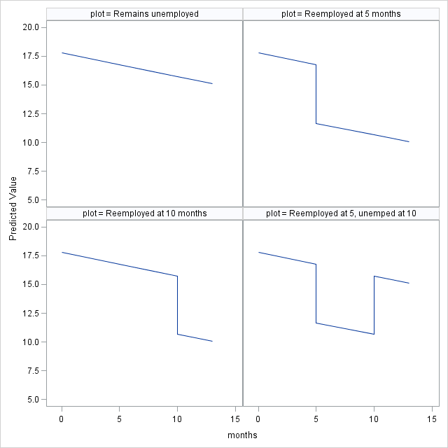
Figure 5.4 on page 167. Based on Model B, Model C and Model D, we generate predicted values for unemp = 0 and unemp =1 cases. The rest is to set up the options to plot each one of them against the time variable. A lot of the code is for setting up the titles, legend and combining the three plots into one.
title;
proc format ;
  value plot 1 = "Model B: Main effects"
             2 = "Model C: Interaction"
             3 = "Model D: Constraint";
run;

data preddata;
do i = 0 to 14;
	months = i;
	unemp = 0;
	output;
end;
do i = 0 to 14;
	months = i;
	unemp = 1;
	output;
end;
run;

*model B;
proc mixed data = unemployment_pp method = ml;
class id;
model cesd  = months unemp/ solution;
random intercept months / subject = id type = un;
store out = bplm;
run;

proc plm source = bplm;
score data = preddata out = bplot;
run;

data bplot;
set bplot;
plot = 1;
run;

*model C;
proc mixed data = unemployment_pp method = ml;
class id;
model cesd  = months|unemp / solution;
random intercept months / subject = id type = un;
store out = cplm;
run;

proc plm source = cplm;
score data = preddata out = cplot;
run;

data cplot;
set cplot;
plot = 2;
run;

*model D;
proc mixed data = unemployment_pp method = ml;
class id;
model cesd  = unemp unemp*months / solution;
random intercept unemp months*unemp / subject = id type = un;
store out = dplm;
run;

proc plm source = dplm;
score data = preddata out = dplot;
run;

*plot;
data dplot;
set dplot;
plot = 3;
run;

data fig53;
set bplot cplot dplot;
format plot plot.;
run;

proc sgpanel data = fig53;
panelby plot / layout = columnlattice;
series x = months y = Predicted / group = unemp;
rowaxis max = 20 min = 5 label = "CES-D";
colaxis min = -1 max = 15 label = "Months since job loss";
run;
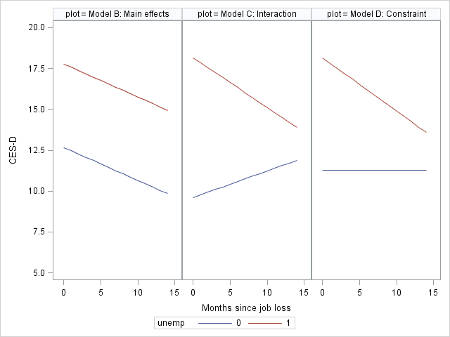
Table 5.8 on page 175.
title1 'Table 5.8: High school dropout wage data--Effects of time-varying unemployment rate';
proc mixed data='c:\alda\wages_pp' method=ml covtest noclprint noinfo;
  title2 'Model A: Unemployment rate centered around 7';
  class id;
  model lnw=hgc_9 ue_7 exper black*exper / solution notest;
  random intercept exper/subject=id type=un;
run;

proc mixed data='c:\alda\wages_pp' method=ml covtest noclprint noinfo;
  title2 'Model B: Within context centering';
  class id;
  model lnw=hgc_9 ue_mean ue_person_centered exper black*exper / solution notest;
  random intercept exper/subject=id type=un;
run;

proc mixed data='c:\alda\wages_pp' method=ml covtest noclprint noinfo;
  title2 'Model C: Centering on time-1';
  class id;
  model lnw=hgc_9 ue1 ue_centert1 exper black*exper / solution notest;
  random intercept exper / subject=id type=un;
run;
Table 5.8: High school dropout wage data--Effects of time-varying unemployment rate
Model A: Unemployment rate centered around 7
The Mixed Procedure
                  Covariance Parameter Estimates
Standard Z Cov Parm Subject Estimate Error Value Pr Z UN(1,1) ID 0.05064 0.004808 10.53 <.0001 UN(2,1) ID -0.00291 0.000838 -3.47 0.0005 UN(2,2) ID 0.001631 0.000213 7.68 <.0001 Residual 0.09480 0.001938 48.91 <.0001
Fit Statistics -2 Log Likelihood 4830.5 AIC (smaller is better) 4848.5 AICC (smaller is better) 4848.5 BIC (smaller is better) 4891.6
  Null Model Likelihood Ratio Test
    DF    Chi-Square      Pr > ChiSq
     3       1423.34          <.0001
Solution for Fixed Effects
Standard Effect Estimate Error DF t Value Pr > |t| Intercept 1.7490 0.01140 886 153.43 <.0001 HGC_9 0.04001 0.006363 4662 6.29 <.0001 UE_7 -0.01195 0.001792 4662 -6.67 <.0001 EXPER 0.04405 0.002603 849 16.92 <.0001 EXPER*BLACK -0.01818 0.004483 4662 -4.06 <.0001
Table 5.8: High school dropout wage data--Effects of time-varying unemployment r
Model B: Within context centering
The Mixed Procedure
Covariance Parameter Estimates
Standard Z Cov Parm Subject Estimate Error Value Pr Z UN(1,1) ID 0.05101 0.004841 10.54 <.0001 UN(2,1) ID -0.00302 0.000843 -3.59 0.0003 UN(2,2) ID 0.001628 0.000212 7.67 <.0001 Residual 0.09480 0.001938 48.91 <.0001
           Fit Statistics
-2 Log Likelihood              4827.0
AIC (smaller is better)        4847.0
AICC (smaller is better)       4847.0
BIC (smaller is better)        4894.9
  Null Model Likelihood Ratio Test
    DF    Chi-Square      Pr > ChiSq
     3       1407.18          <.0001
Solution for Fixed Effects
Standard Effect Estimate Error DF t Value Pr > |t| Intercept 1.8743 0.02952 885 63.48 <.0001 HGC_9 0.04017 0.006351 4662 6.33 <.0001 UE_MEAN -0.01771 0.003520 4662 -5.03 <.0001 UE_PERSON_CENTERED -0.00990 0.002097 4662 -4.72 <.0001 EXPER 0.04506 0.002650 849 17.00 <.0001 EXPER*BLACK -0.01887 0.004477 4662 -4.22 <.0001
Table 5.8: High school dropout wage data--Effects of time-varying unemployment r
Model C: Centering on time-1
The Mixed Procedure
Covariance Parameter Estimates
Standard Z Cov Parm Subject Estimate Error Value Pr Z UN(1,1) ID 0.05028 0.004789 10.50 <.0001 UN(2,1) ID -0.00290 0.000838 -3.46 0.0005 UN(2,2) ID 0.001635 0.000213 7.68 <.0001 Residual 0.09477 0.001937 48.92 <.0001
           Fit Statistics
-2 Log Likelihood              4825.8
AIC (smaller is better)        4845.8
AICC (smaller is better)       4845.9
BIC (smaller is better)        4893.7
  Null Model Likelihood Ratio Test
    DF    Chi-Square      Pr > ChiSq
     3       1423.82          <.0001
Solution for Fixed Effects
Standard Effect Estimate Error DF t Value Pr > |t| Intercept 1.8693 0.02603 886 71.81 <.0001 HGC_9 0.03993 0.006349 4661 6.29 <.0001 UE1 -0.01618 0.002648 4661 -6.11 <.0001 UE_CENTERT1 -0.01031 0.001944 4661 -5.30 <.0001 EXPER 0.04476 0.002625 849 17.06 <.0001 EXPER*BLACK -0.01832 0.004484 4661 -4.09 <.0001
Table 5.10 on page 184.
title1 'Table 5.10: Alternative parameterizations for the main effect
        of TIME in the antidepressant trial';
proc mixed data='c:\alda\medication_pp' noclprint noinfo method=ml covtest;
  title2 'Model A: TIME';
  class id;
  model pos = treat time treat*time / solution ddfm=bw notest;
  random intercept time / subject=id type=un;
run;

proc mixed data='c:\alda\medication_pp' noclprint noinfo Method=ml covtest;
  title2 'Model B: TIME-3.33';
  class id;
  model pos = treat time333 treat*time333 / solution ddfm=bw notest;
  random intercept time333 / subject=id type=un;
	run;

proc mixed data='c:\alda\medication_pp' noclprint noinfo Method=ml covtest;
  title2 'Model C: TIME-6.67';
  class id;
  model pos = treat time667 treat*time667 / solution ddfm=bw notest;
  random intercept time667 / subject=id type=un;
run;

Table 5.10: Alternative parameterizations for the main effect of TIME in the ant
Model A: TIME
                Covariance Parameter Estimates

                                    Standard         Z
Cov Parm     Subject    Estimate       Error     Value        Pr Z
UN(1,1)      ID          2111.33      420.19      5.02      <.0001
UN(2,1)      ID          -121.62     59.0314     -2.06      0.0394
UN(2,2)      ID          63.7351     14.2712      4.47      <.0001
Residual                 1229.93     52.0915     23.61      <.0001
           Fit Statistics
-2 Log Likelihood             12680.5
AIC (smaller is better)       12696.5
AICC (smaller is better)      12696.6
BIC (smaller is better)       12713.7
  Null Model Likelihood Ratio Test
    DF    Chi-Square      Pr > ChiSq
     3        971.31          <.0001
Solution for Fixed Effects
Standard Effect Estimate Error DF t Value Pr > |t| Intercept 167.46 9.3261 62 17.96 <.0001 TREAT -3.1093 12.3324 62 -0.25 0.8018 TIME -2.4181 1.7308 1176 -1.40 0.1627 TREAT*TIME 5.5368 2.2778 1176 2.43 0.0152
Table 5.10: Alternative parameterizations for the main effect of TIME in the ant
Model B: TIME-3.33
The Mixed Procedure
Covariance Parameter Estimates
Standard Z Cov Parm Subject Estimate Error Value Pr Z UN(1,1) ID 2008.72 367.24 5.47 <.0001 UN(2,1) ID 90.8341 52.4581 1.73 0.0834 UN(2,2) ID 63.7351 14.2712 4.47 <.0001 Residual 1229.93 52.0915 23.61 <.0001
           Fit Statistics
-2 Log Likelihood             12680.5
AIC (smaller is better)       12696.5
AICC (smaller is better)      12696.6
BIC (smaller is better)       12713.7
  Null Model Likelihood Ratio Test
    DF    Chi-Square      Pr > ChiSq
     3        971.31          <.0001
Solution for Fixed Effects
Standard Effect Estimate Error DF t Value Pr > |t| Intercept 159.40 8.7644 62 18.19 <.0001 TREAT 15.3467 11.5445 62 1.33 0.1886 TIME333 -2.4181 1.7308 1176 -1.40 0.1627 TREAT*TIME333 5.5368 2.2778 1176 2.43 0.0152
Table 5.10: Alternative parameterizations for the main effect of TIME in the ant
Model C: TIME-6.67
The Mixed Procedure
Covariance Parameter Estimates
Standard Z Cov Parm Subject Estimate Error Value Pr Z UN(1,1) ID 3322.45 632.11 5.26 <.0001 UN(2,1) ID 303.28 80.9007 3.75 0.0002 UN(2,2) ID 63.7351 14.2712 4.47 <.0001 Residual 1229.93 52.0915 23.61 <.0001
           Fit Statistics
-2 Log Likelihood             12680.5
AIC (smaller is better)       12696.5
AICC (smaller is better)      12696.6
BIC (smaller is better)       12713.7
  Null Model Likelihood Ratio Test
    DF    Chi-Square      Pr > ChiSq
     3        971.31          <.0001
Solution for Fixed Effects
Standard Effect Estimate Error DF t Value Pr > |t| Intercept 151.34 11.5424 62 13.11 <.0001 TREAT 33.8028 15.1580 62 2.23 0.0294 TIME667 -2.4181 1.7308 1176 -1.40 0.1627 TREAT*TIME667 5.5368 2.2778 1176 2.43 0.0152
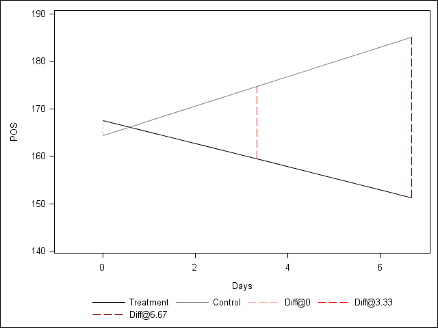
Figure 5.5 on page 185.
data preddata;
input time treat line $16. ;
datalines;
0 0 Treatment
3.33 0 Treatment
6.67 0 Treatment
0 1 Control
3.33 1 Control
6.67 1 Control
0 0 Diff@0
0 1 Diff@0
3.33 0 Diff@3.33
3.33 1 Diff@3.33
6.67 0 Diff@6.67
6.67 1 Diff@6.67
;
run;

proc mixed data = medication_pp method = ml;
class id;
model pos = treat|time / solution;
random intercept time / subject = id type=un;
store out=medplm;
run;

proc plm source = medplm;
score out = medplot data = preddata;
run;

proc template;
define style newstyle;
	style GraphData1 /
		LineStyle = 1
		Contrastcolor = black;
	style GraphData2 /
		LineStyle = 1
		Contrastcolor = gray;
	style GraphData3  /
		LineStyle = 4
		Contrastcolor = very light red;
	style GraphData4 from GraphData3  /
		Contrastcolor = red;
	style GraphData5  from GraphData3 /
		Contrastcolor = very dark red;
end;
run;

ods html style = newstyle;

proc sgplot data = medplot noautolegend;
series x = time y = Predicted / group = line;
xaxis min = -1 max = 7 label = "Days";
yaxis min = 140 max = 190 label = "POS";
keylegend / noborder location = outside;
run;
Page 188 on modeling initial and final status.
proc mixed data='c:\alda\medication_pp' noclprint noinfo Method=ml covtest;
  title2 'Model in Text: Initial and final status model';
  class id;
  model pos = Initial treat*initial final treat*final / solution noint ddfm=bw notest;
  random initial final / subject=id type=un gcorr;
run;

Model in Text: Initial and final status model
The Mixed Procedure
Iteration History
Iteration Evaluations -2 Log Like Criterion
        0              1     13651.76032736
        1              2     12680.45210673      0.00000011
        2              1     12680.45155817      0.00000000
Convergence criteria met.
Estimated G Correlation Matrix
Row Effect ID Col1 Col2
   1    INITIAL      1      1.0000      0.4910
   2    FINAL        1      0.4910      1.0000
Covariance Parameter Estimates
Standard Z Cov Parm Subject Estimate Error Value Pr Z
UN(1,1)      ID          2111.33      420.19      5.02      <.0001
UN(2,1)      ID          1300.56      392.77      3.31      0.0009
UN(2,2)      ID          3322.45      632.11      5.26      <.0001
Residual                 1229.93     52.0915     23.61      <.0001
Fit Statistics
-2 Log Likelihood             12680.5
AIC (smaller is better)       12696.5
AICC (smaller is better)      12696.6
BIC (smaller is better)       12713.7
Null Model Likelihood Ratio Test
DF Chi-Square Pr > ChiSq
3 971.31 <.0001
Solution for Fixed Effects
Standard Effect Estimate Error DF t Value Pr > |t|
INITIAL            167.46      9.3261    1174      17.96      <.0001
INITIAL*TREAT     -3.1093     12.3324    1174      -0.25      0.8010
FINAL              151.34     11.5424    1174      13.11      <.0001
TREAT*FINAL       33.8028     15.1580    1174       2.23      0.0259

