Note: This page has been updated SAS 9.3 and is based partly on SAS 9.2code provided by Raymond R. Balise of Stanford University. We thank Raymond R. Balise for sharing his SAS 9.2 code with us.
Table 6.1 on page 192.
title1 'Table 6.1: Excerpts from person-period data set for high school dropout study';
proc print data='c:\alda\wages_pp';
  where id in (206,2365,4384);
  id id;
  var lnw exper ged postexp;
run;

Table 6.1: Excerpts from person-period data set for high school dropout study
 ID      LNW      EXPER    GED    POSTEXP
 206    2.028     1.874     0      0.000
 206    2.297     2.814     0      0.000
 206    2.482     4.314     0      0.000
2365    1.782     0.660     0      0.000
2365    1.763     1.679     0      0.000
2365    1.710     2.737     0      0.000
2365    1.736     3.679     0      0.000
2365    2.192     4.679     1      0.000
2365    2.042     5.718     1      1.038
2365    2.320     6.718     1      2.038
2365    2.665     7.872     1      3.192
2365    2.418     9.083     1      4.404
2365    2.389    10.045     1      5.365
2365    2.485    11.122     1      6.442
2365    2.445    12.045     1      7.365
4384    2.859     0.096     0      0.000
4384    1.532     1.039     0      0.000
4384    1.590     1.726     1      0.000
4384    1.969     3.128     1      1.402
4384    1.684     4.282     1      2.556
4384    2.625     5.724     1      3.998
4384    2.583     6.024     1      4.298
Figure 6.1. We use id = 53 for the purpose of illustration. The plot here is not exactly the same as in the book, but it has the same features.
proc mixed data=wages_pp method=ml noclprint noinfo;
  class id;
  model lnw=exper / solution notest outpm = ma;
  random intercept exper / subject=id type=un;
run;
proc mixed data=wages_pp  method=ml noclprint noinfo;
  class id;
  model lnw=exper ged / solution notest outpm = mb;
  random intercept exper ged / subject=id type=un;
run;
proc mixed data=wages_pp  method=ml noclprint noinfo;
  class id;
  model lnw=exper postexp / solution notest outpm = mc;
  random intercept exper / subject=id type=un;
run;
proc mixed data=wages_pp  method=ml noclprint noinfo;
  class id;
  model lnw=exper ged postexp /solution notest outpm = md;
  random intercept exper ged postexp / subject=id type=un;
run;
data all;
  merge ma  (where =(id=53) rename=(pred=p1))
        mb  (where =(id=53) rename=(pred=p2))
        mc  (where =(id=53) rename=(pred=p3))
        md  (where =(id=53) rename=(pred=p4));
run;
ods graphics on  / height=3.5in width=4.5in;
proc sgplot data = all;
  series x = exper y = p1 /legendlabel = "A" lineattrs = (color = black pattern = 1 thickness =1);
  series x = exper y = p2 /legendlabel = "B" lineattrs = (color = black pattern = 2 thickness =2);
  series x = exper y = p3 /legendlabel = "C" lineattrs = (color = black pattern = 3 thickness =2);
  series x = exper y = p4 /legendlabel = "D" lineattrs = (color = black pattern = 4 thickness =2);
  keylegend  /noborder location = inside position = bottomright;
run;
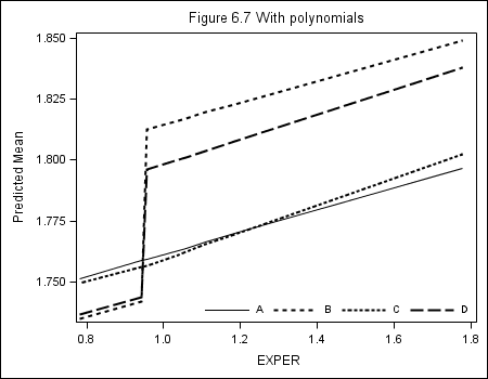
Table 6.2, page 203
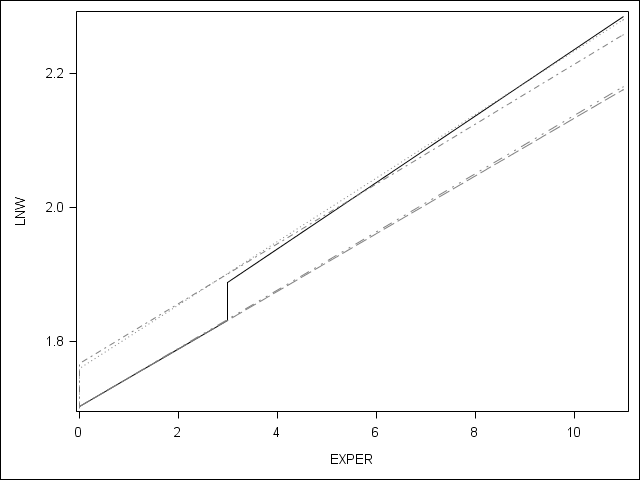
Figure 6.2. Here we plot prototypical (predicted) trajectories. The plots here are not exactly the same as in the book, but have the same features. Additionally, because these plots use different predictors, it requires a GREAT deal more code to get all 4 plots into 1 single panel plot, so we present code for separate plots.
proc template; define style newstyle; style GraphData1/ LineStyle = 1 Contrastcolor = black; style GraphData2/ LineStyle = 4 Contrastcolor = gray; style GraphData3/ LineStyle = 15 Contrastcolor = gray; style GraphData4/ LineStyle = 34 Contrastcolor = gray; style GraphData5/ LineStyle = 41 Contrastcolor = gray; end; run; ods html style = newstyle; *topleft; data preddata; input exper ged line; datalines; 0 0 1 3 0 1 3 1 1 11 1 1 0 0 2 3 0 2 3 0 2 11 0 2 ; run; proc mixed data=wages_pp method=ml noclprint noinfo; model lnw = exper ged; random intercept exper / subject = id type = un; store out = plm; run; proc plm source = plm; score data = preddata out = plot; run; proc sgplot data = plot noautolegend; series x = exper y = Predicted / group = line; xaxis label = "EXPER"; yaxis label = "LNW"; run;*top right; data preddata; input exper ged postexp line; datalines; 0 0 0 1 3 0 0 1 3 1 0 1 11 1 8 1 0 0 0 2 3 0 0 2 3 0 0 2 11 0 0 2 ; run; proc mixed data=wages_pp method=ml noclprint noinfo; model lnw = exper postexp; random intercept exper / subject = id type = un; store out = plm; run; proc plm source = plm; score data = preddata out = plot; run; proc sgplot data = plot noautolegend; series x = exper y = Predicted / group = line; xaxis label = "EXPER"; yaxis label = "LNW"; run;
*bottom left; data preddata; input exper ged postexp line; datalines; 0 0 0 1 3 0 0 1 3 1 0 1 11 1 8 1 0 0 0 2 3 0 0 2 3 1 0 2 11 1 0 2 0 0 0 3 3 0 0 3 3 0 0 3 11 0 0 3 ; run; proc mixed data=wages_pp method=ml noclprint noinfo; model lnw = exper postexp ged; random intercept exper / subject = id type = un; store out = plm; run; proc plm source = plm; score data = preddata out = plot; run; proc sgplot data = plot noautolegend; series x = exper y = Predicted / group = line; xaxis label = "EXPER"; yaxis label = "LNW"; run;
*bottom right; data preddata; input exper ged postexp line; datalines; 0 0 0 1 3 0 0 1 3 1 0 1 11 1 8 1 0 0 0 2 3 0 0 2 3 0 0 2 11 0 0 2 ; run; proc mixed data=wages_pp method=ml noclprint noinfo; model lnw = exper postexp ged; random intercept exper / subject = id type = un; store out = plm; run; proc plm source = plm; score data = preddata out = aplot; run; data preddata; input exper ged postexp line; datalines; 0 0 0 3 11 0 0 3 0 0 0 4 0 1 0 4 11 1 0 4 ; run; proc mixed data=wages_pp method=ml noclprint noinfo; model lnw = exper|ged; random intercept exper / subject = id type = un; store out = plm; run; proc plm source = plm; score data = preddata out = bplot; run; data preddata; input exper ged postexp line; datalines; 0 0 0 5 0 1 0 5 11 1 0 5 ; run; proc mixed data=wages_pp method=ml noclprint noinfo; model lnw = exper ged; random intercept exper / subject = id type = un; store out = plm; run; proc plm source = plm; score data = preddata out = cplot; run; data plot; set aplot bplot cplot; run; proc sgplot data = plot noautolegend; series x = exper y = Predicted / group = line; xaxis label = "EXPER"; yaxis label = "LNW"; run;
title1 'Table 6.2: Alternative discontinuous change trajectories: HS dropout data';
proc mixed data='c:\alda\wages_pp' method=ml noclprint noinfo;
  title2 'Model A: EXPER, HGC-9, BLACK*EXPER, UE-7';
  class id;
  model lnw=exper hgc_9 exper*black ue_7 / solution notest;
  random intercept exper / subject=id type=un;
run;

proc mixed data='c:\alda\wages_pp' method=ml noclprint noinfo;
  title2 'Model B: A + GED as fixed and random effect';
  class id;
  model lnw=exper hgc_9 exper*black ue_7 ged / solution notest;
  random intercept exper ged / subject=id type=un;
run;

proc mixed data='c:\alda\wages_pp' method=ml noclprint noinfo;
  title2 'Model C: Model B without random effect of GED ';
  class id;
  model lnw=exper hgc_9 exper*black ue_7 ged / solution notest;
  random intercept exper / subject=id type=un;
run;

proc mixed data='c:\alda\wages_pp' method=ml noclprint noinfo;
  title2 'Model D: A + POSTEXP as fixed and random effect';
  class id;
  model lnw=exper hgc_9 exper*black ue_7 postexp /solution notest;
  random intercept exper postexp / subject=id type=un;
run;

proc mixed data='c:\alda\wages_pp' method=ml noclprint noinfo;
  title2 'Model E: Model D without random effect of POSTEXP ';
  class id;
  model lnw=exper hgc_9 exper*black ue_7 postexp / solution notest;
  random intercept exper / subject=id type=un;
run;

proc mixed data='c:\alda\wages_pp' method=ml noclprint noinfo;
  title2 'Model F: Model A with fixed and random effects of GED and POSTEXP ';
  class id;
  model lnw=exper hgc_9 exper*black ue_7 ged postexp / solution notest;
  random intercept exper ged postexp / subject=id type=un;
run;

proc mixed data='c:\alda\wages_pp' method=ml noclprint noinfo;
  title2 'Model G: Model F without random effect of POSTEXP ';
  class id;
  model lnw=exper hgc_9 exper*black ue_7 ged postexp / solution notest;
  random intercept exper ged / subject=id type=un;
run;

proc mixed data='c:\alda\wages_pp' method=ml noclprint noinfo;
  title2 'Model H: Model F without random effect of GED';
  class id;
  model lnw=exper hgc_9 exper*black ue_7 ged postexp / solution notest;
  random intercept exper postexp / subject=id type=un;
run;

proc mixed data='c:\alda\wages_pp' method=ml noclprint noinfo;
  title2 'Model I: Model A with GED and GED*EXPER as fixed and random effects';
  class id;
  model lnw=exper hgc_9 exper*black ue_7 ged ged*exper / solution notest;
  random intercept exper ged ged*exper / subject=id type=un;
run;

proc mixed data='c:\alda\wages_pp' method=ml noclprint noinfo;
  title2 'Model J: Model I without random effect of GED*EXPER';
  class id;
  model lnw=exper hgc_9 exper*black ue_7 ged ged*exper / solution notest;
  random intercept exper ged / subject=id type=un;
run;

Table 6.2: Alternative discontinuous change trajectories: HS dropout data
Model A: EXPER, HGC-9, BLACK*EXPER, UE-7
The Mixed ProcedureCovariance Parameter Estimates
Cov Parm Subject Estimate
UN(1,1)      ID          0.05064
UN(2,1)      ID         -0.00291
UN(2,2)      ID         0.001631
Residual                 0.09480
Fit Statistics
-2 Log Likelihood              4830.5
AIC (smaller is better)        4848.5
AICC (smaller is better)       4848.5
BIC (smaller is better)        4891.6
  Null Model Likelihood Ratio Test
    DF    Chi-Square      Pr > ChiSq
     3       1423.34          <.0001
Solution for Fixed EffectsStandard Effect Estimate Error DF t Value Pr > |t| Intercept 1.7490 0.01140 886 153.43 <.0001 EXPER 0.04405 0.002603 849 16.92 <.0001 HGC_9 0.04001 0.006363 4662 6.29 <.0001 EXPER*BLACK -0.01818 0.004483 4662 -4.06 <.0001 UE_7 -0.01195 0.001792 4662 -6.67 <.0001
Table 6.2: Alternative discontinuous change trajectories: HS dropout data
Model B: A + GED as fixed and random effect
The Mixed Procedure
Covariance Parameter EstimatesCov Parm Subject Estimate UN(1,1) ID 0.04360 UN(2,1) ID -0.00262 UN(2,2) ID 0.001660 UN(3,1) ID 0.002341 UN(3,2) ID -0.00218 UN(3,3) ID 0.02824 Residual 0.09416
           Fit Statistics
-2 Log Likelihood              4805.5
AIC (smaller is better)        4831.5
AICC (smaller is better)       4831.6
BIC (smaller is better)        4893.8
  Null Model Likelihood Ratio Test
    DF    Chi-Square      Pr > ChiSq
     6       1410.01          <.0001
Solution for Fixed EffectsStandard Effect Estimate Error DF t Value Pr > |t| Intercept 1.7342 0.01180 886 146.97 <.0001 EXPER 0.04322 0.002621 849 16.49 <.0001 HGC_9 0.03833 0.006265 4558 6.12 <.0001 EXPER*BLACK -0.01820 0.004470 4558 -4.07 <.0001 UE_7 -0.01161 0.001788 4558 -6.49 <.0001 GED 0.06131 0.01845 103 3.32 0.0012
Table 6.2: Alternative discontinuous change trajectories: HS dropout data
Model C: Model B without random effect of GED
The Mixed Procedure
Covariance Parameter EstimatesCov Parm Subject Estimate
UN(1,1) ID 0.05058 UN(2,1) ID -0.00304 UN(2,2) ID 0.001634 Residual 0.09474
Fit Statistics -2 Log Likelihood 4818.3 AIC (smaller is better) 4838.3 AICC (smaller is better) 4838.4 BIC (smaller is better) 4886.2
Null Model Likelihood Ratio Test
DF Chi-Square Pr > ChiSq
3 1397.20 <.0001
Solution for Fixed EffectsStandard Effect Estimate Error DF t Value Pr > |t| Intercept 1.7343 0.01213 886 142.93 <.0001 EXPER 0.04333 0.002608 849 16.61 <.0001 HGC_9 0.03904 0.006334 4661 6.16 <.0001 EXPER*BLACK -0.01852 0.004460 4661 -4.15 <.0001 UE_7 -0.01159 0.001793 4661 -6.47 <.0001 GED 0.05912 0.01687 4661 3.51 0.0005
Table 6.2: Alternative discontinuous change trajectories: HS dropout data Model D: A + POSTEXP as fixed and random effect
The Mixed Procedure
Covariance Parameter EstimatesCov Parm Subject Estimate UN(1,1) ID 0.05056 UN(2,1) ID -0.00245 UN(2,2) ID 0.001448 UN(3,1) ID -0.00201 UN(3,2) ID -0.00005 UN(3,3) ID 0.000880 Residual 0.09464
Fit Statistics -2 Log Likelihood 4817.4 AIC (smaller is better) 4843.4 AICC (smaller is better) 4843.4 BIC (smaller is better) 4905.6
Null Model Likelihood Ratio Test
DF Chi-Square Pr > ChiSq
6 1390.91 <.0001
Solution for Fixed Effects
Standard
Effect Estimate Error DF t Value Pr > |t|
Intercept 1.7494 0.01140 886 153.47 <.0001
EXPER 0.04065 0.002777 849 14.64 <.0001
HGC_9 0.03988 0.006354 4545 6.28 <.0001
EXPER*BLACK -0.01949 0.004474 4545 -4.36 <.0001
UE_7 -0.01184 0.001791 4545 -6.61 <.0001
POSTEXP 0.01459 0.004564 116 3.20 0.0018
Table 6.2: Alternative discontinuous change trajectories: HS dropout data Model E: Model D without random effect of POSTEXP
The Mixed Procedure
Covariance Parameter EstimatesCov Parm Subject Estimate UN(1,1) ID 0.05085 UN(2,1) ID -0.00304 UN(2,2) ID 0.001612 Residual 0.09484
Fit Statistics -2 Log Likelihood 4820.7 AIC (smaller is better) 4840.7 AICC (smaller is better) 4840.7 BIC (smaller is better) 4888.6
Null Model Likelihood Ratio Test
DF Chi-Square Pr > ChiSq
3 1387.58 <.0001
Solution for Fixed EffectsStandard Effect Estimate Error DF t Value Pr > |t| Intercept 1.7499 0.01141 886 153.35 <.0001 EXPER 0.04051 0.002828 849 14.32 <.0001 HGC_9 0.03954 0.006334 4661 6.24 <.0001 EXPER*BLACK -0.01918 0.004452 4661 -4.31 <.0001 UE_7 -0.01185 0.001791 4661 -6.62 <.0001 POSTEXP 0.01396 0.004423 4661 3.16 0.0016
Table 6.2: Alternative discontinuous change trajectories: HS dropout data Model F: Model A with fixed and random effects of GED and POSTEXP
The Mixed Procedure
Covariance Parameter EstimatesCov Parm Subject Estimate UN(1,1) ID 0.04132 UN(2,1) ID -0.00170 UN(2,2) ID 0.001360 UN(3,1) ID 0.01196 UN(3,2) ID 0.002931 UN(3,3) ID 0.01631 UN(4,1) ID -0.00605 UN(4,2) ID -0.00091 UN(4,3) ID -0.00391 UN(4,4) ID 0.003355 Residual 0.09387
Fit Statistics -2 Log Likelihood 4789.4 AIC (smaller is better) 4825.4 AICC (smaller is better) 4825.5 BIC (smaller is better) 4911.6
Null Model Likelihood Ratio Test
DF Chi-Square Pr > ChiSq
10 1416.42 <.0001
Solution for Fixed EffectsStandard Effect Estimate Error DF t Value Pr > |t| Intercept 1.7386 0.01194 886 145.59 <.0001 EXPER 0.04147 0.002797 849 14.83 <.0001 HGC_9 0.03903 0.006243 4468 6.25 <.0001 EXPER*BLACK -0.01962 0.004470 4468 -4.39 <.0001 UE_7 -0.01172 0.001783 4468 -6.58 <.0001 GED 0.04088 0.02199 103 1.86 0.0659 POSTEXP 0.009422 0.005545 89 1.70 0.0928
Table 6.2: Alternative discontinuous change trajectories: HS dropout data Model G: Model F without random effect of POSTEXP
The Mixed Procedure
Covariance Parameter EstimatesCov Parm Subject Estimate UN(1,1) ID 0.04349 UN(2,1) ID -0.00258 UN(2,2) ID 0.001651 UN(3,1) ID 0.002534 UN(3,2) ID -0.00235 UN(3,3) ID 0.02850 Residual 0.09417
Fit Statistics -2 Log Likelihood 4802.7 AIC (smaller is better) 4830.7 AICC (smaller is better) 4830.8 BIC (smaller is better) 4897.7
Null Model Likelihood Ratio Test
DF Chi-Square Pr > ChiSq
6 1403.08 <.0001
Solution for Fixed EffectsStandard Effect Estimate Error DF t Value Pr > |t| Intercept 1.7389 0.01211 886 143.56 <.0001 EXPER 0.04117 0.002884 849 14.27 <.0001
Solution for Fixed EffectsStandard Effect Estimate Error DF t Value Pr > |t| HGC_9 0.03831 0.006263 4557 6.12 <.0001 EXPER*BLACK -0.01871 0.004470 4557 -4.18 <.0001 UE_7 -0.01164 0.001787 4557 -6.51 <.0001 GED 0.04307 0.02136 103 2.02 0.0464 POSTEXP 0.008663 0.005120 4557 1.69 0.0907
Table 6.2: Alternative discontinuous change trajectories: HS dropout data Model H: Model F without random effect of GED
The Mixed Procedure
Covariance Parameter EstimatesCov Parm Subject Estimate UN(1,1) ID 0.05037 UN(2,1) ID -0.00247 UN(2,2) ID 0.001452 UN(3,1) ID -0.00192 UN(3,2) ID 4.994E-6 UN(3,3) ID 0.000757 Residual 0.09458
Fit Statistics -2 Log Likelihood 4812.6 AIC (smaller is better) 4840.6 AICC (smaller is better) 4840.7 BIC (smaller is better) 4907.7
Null Model Likelihood Ratio Test
DF Chi-Square Pr > ChiSq
6 1393.13 <.0001
Solution for Fixed Effects
Standard
Effect Estimate Error DF t Value Pr > |t|
Intercept 1.7386 0.01242 886 139.98 <.0001
EXPER 0.04147 0.002804 849 14.79 <.0001
HGC_9 0.03935 0.006351 4544 6.20 <.0001
EXPER*BLACK -0.01935 0.004477 4544 -4.32 <.0001
UE_7 -0.01162 0.001792 4544 -6.49 <.0001
GED 0.04251 0.01949 4544 2.18 0.0292
POSTEXP 0.008554 0.005329 116 1.61 0.1112
Table 6.2: Alternative discontinuous change trajectories: HS dropout data Model I: Model A with GED and GED*EXPER as fixed and random effects
The Mixed Procedure
Covariance Parameter EstimatesCov Parm Subject Estimate
UN(1,1) ID 0.04096 UN(2,1) ID -0.00178 UN(2,2) ID 0.001378 UN(3,1) ID -0.01729 UN(3,2) ID 0.02813 UN(3,3) ID 0.08762 UN(4,1) ID 0.000295 UN(4,2) ID -0.00348 UN(4,3) ID -0.03597 UN(4,4) ID 0.008343 Residual 0.09382
Fit Statistics -2 Log Likelihood 4787.0 AIC (smaller is better) 4823.0 AICC (smaller is better) 4823.1 BIC (smaller is better) 4909.2Null Model Likelihood Ratio Test DF Chi-Square Pr > ChiSq 10 1424.80 <.0001
Solution for Fixed EffectsStandard Effect Estimate Error DF t Value Pr > |t| Intercept 1.7386 0.01219 886 142.65 <.0001 EXPER 0.04179 0.002864 849 14.59 <.0001 HGC_9 0.03822 0.006239 4496 6.13 <.0001 EXPER*BLACK -0.01913 0.004471 4496 -4.28 <.0001 UE_7 -0.01194 0.001785 4496 -6.69 <.0001 GED 0.04504 0.02579 103 1.75 0.0837 EXPER*GED 0.005485 0.005512 61 1.00 0.3237
Table 6.2: Alternative discontinuous change trajectories: HS dropout data Model J: Model I without random effect of GED*EXPER
The Mixed ProcedureCovariance Parameter Estimates
Cov Parm Subject Estimate
UN(1,1) ID 0.04363 UN(2,1) ID -0.00261 UN(2,2) ID 0.001655 UN(3,1) ID 0.001676 UN(3,2) ID -0.00222 UN(3,3) ID 0.02956 Residual 0.09416
Fit Statistics -2 Log Likelihood 4804.6 AIC (smaller is better) 4832.6 AICC (smaller is better) 4832.7 BIC (smaller is better) 4899.6
Null Model Likelihood Ratio Test
DF Chi-Square Pr > ChiSq
6 1407.21 <.0001
Solution for Fixed Effects
Standard
Effect Estimate Error DF t Value Pr > |t|
Intercept 1.7378 0.01239 886 140.29 <.0001
EXPER 0.04188 0.002972 849 14.09 <.0001
HGC_9 0.03827 0.006264 4557 6.11 <.0001
EXPER*BLACK -0.01833 0.004467 4557 -4.10 <.0001
UE_7 -0.01163 0.001788 4557 -6.50 <.0001
GED 0.04571 0.02470 103 1.85 0.0671
EXPER*GED 0.004872 0.005064 4557 0.96 0.3360
Table 6.3 on page 205.
title1 'Table 6.3: Model F (with discontinuities in elevation and slope)'; title2 'HS dropout wage data'; proc mixed data='c:\alda\wages_pp' method=ml noclprint noinfo covtest; class id; model lnw=exper hgc_9 exper*black ue_7 ged postexp / solution notest; random intercept exper ged postexp / subject=id type=un; run;
Table 6.3: Model F (with discontinuities in elevation and slope) HS dropout wage data
The Mixed Procedure
Covariance Parameter EstimatesStandard Z Cov Parm Subject Estimate Error Value Pr Z UN(1,1) ID 0.04132 0.004747 8.71 <.0001 UN(2,1) ID -0.00170 0.000826 -2.06 0.0393 UN(2,2) ID 0.001360 0.000217 6.26 <.0001 UN(3,1) ID 0.01196 0.009649 1.24 0.2150 UN(3,2) ID 0.002931 0.004098 0.72 0.4745 UN(3,3) ID 0.01631 0.01763 0.93 0.1775 UN(4,1) ID -0.00605 0.002875 -2.10 0.0355 UN(4,2) ID -0.00091 0.001205 -0.76 0.4493 UN(4,3) ID -0.00391 0.004877 -0.80 0.4229 UN(4,4) ID 0.003355 0.002401 1.40 0.0812 Residual 0.09387 0.001933 48.55 <.0001
Fit Statistics -2 Log Likelihood 4789.4 AIC (smaller is better) 4825.4 AICC (smaller is better) 4825.5 BIC (smaller is better) 4911.6
Null Model Likelihood Ratio Test
DF Chi-Square Pr > ChiSq
10 1416.42 <.0001
Solution for Fixed Effects
Standard
Effect Estimate Error DF t Value Pr > |t|
Intercept 1.7386 0.01194 886 145.59 <.0001
EXPER 0.04147 0.002797 849 14.83 <.0001
HGC_9 0.03903 0.006243 4468 6.25 <.0001
EXPER*BLACK -0.01962 0.004470 4468 -4.39 <.0001
UE_7 -0.01172 0.001783 4468 -6.58 <.0001
GED 0.04088 0.02199 103 1.86 0.0659
POSTEXP 0.009422 0.005545 89 1.70 0.0928
Figure 6.3 on page 206
proc format library=mylib;
value fig 1 = 'white/latino 9th'
2 = 'white/latino 12th'
3 = 'black 9th'
4 = 'black 12th';
run;
options fmtsearch = (mylib);
proc template;
define style newstyle;
style GraphData1/
LineStyle = 1
Contrastcolor = gray;
style GraphData2/
LineStyle = 4
Contrastcolor = gray;
style GraphData3/
LineStyle = 1
Contrastcolor = black;
style GraphData4/
LineStyle = 4
Contrastcolor = black;
end;
run;
data preddata;
input exper postexp ged black hgc_9 line;
datalines;
0 0 0 0 0 1
3 0 0 0 0 1
3 0 1 0 0 1
11 8 1 0 0 1
0 0 0 0 3 2
3 0 0 0 3 2
3 0 1 0 3 2
11 8 1 0 3 2
0 0 0 1 0 3
3 0 0 1 0 3
3 0 1 1 0 3
11 8 1 1 0 3
0 0 0 1 3 4
3 0 0 1 3 4
3 0 1 1 3 4
11 8 1 1 3 4
;
run;
data preddata;
set preddata;
format line fig.;
run;
proc mixed data=wages_pp method=ml noclprint noinfo covtest;
class id;
model lnw=exper hgc_9 exper*black ue_7 ged postexp / solution notest;
random intercept exper ged postexp / subject=id type=un;
store out = plm;
run;
proc plm source = plm;
score data = preddata out = plotdata;
run;
proc sgplot data = plotdata;
series x = exper y = predicted / group = line;
keylegend /;
run;
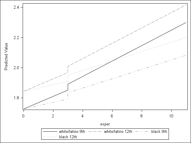
Figure 6.4 on page 209.
PROC SGPANEL does not allow the range of y-axis values to vary by plot, so we present 3 separate plots.
proc format library=mylib;
value fig 1 = 'Raw'
2 = 'IQ^2.3'
3 = 'Age^(1/2.3)';
run;
options fmtsearch = (mylib);
data berkeley_pp;
set "F:/alda/SAS/berkeley_pp";
run;
data berkeley_pp;
set berkeley_pp;
plot = 1;
output;
run;
data berkeley_pp2;
set berkeley_pp;
iq = iq**2.3;
plot = 2;
run;
data berkeley_pp3;
set berkeley_pp;
age = age**(1/2.3);
plot = 3;
run;
data plotdata;
set berkeley_pp berkeley_pp2 berkeley_pp3;
format plot fig.;
run;
proc sgplot data = plotdata;
scatter x = age y = iq / markerattrs=(color=black symbol=circlefilled);
xaxis label = "TIME";
yaxis label = "IQ";
by plot;
run;
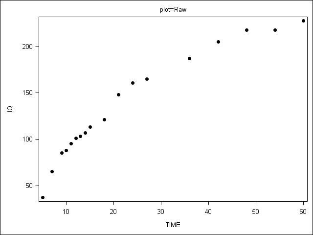
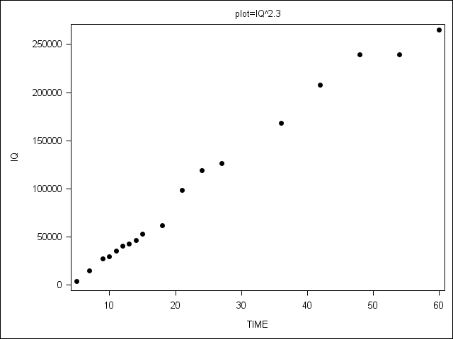
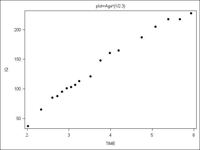
Table 6.4 on page 214.
data table64; do time = 5 to 95; y0 = 71; y1 = 71 + (1.2*time); y2 = 50 + (3.8*time) + (-.03*time*time); y3 = 30 + (10*time) + (-.2*time*time) + (.0012*time*time*time); output; end; run; proc sgplot data = table64; inset "No Change"; series x = time y = y0; yaxis min = 0 max = 200 label="Y"; run; proc sgplot data = table64; inset "Linear Change"; series x = time y = y1; yaxis min = 0 max = 200 label="Y"; run; proc sgplot data = table64; inset "Quadratic Change"; series x = time y = y2; yaxis min = 0 max = 200 label="Y"; run; proc sgplot data = table64; inset "Cubic Change"; series x = time y = y3; yaxis min = 0 max = 200 label="Y"; run;
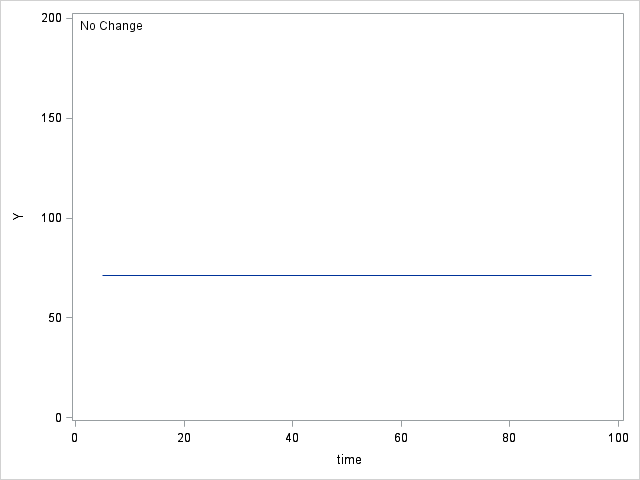
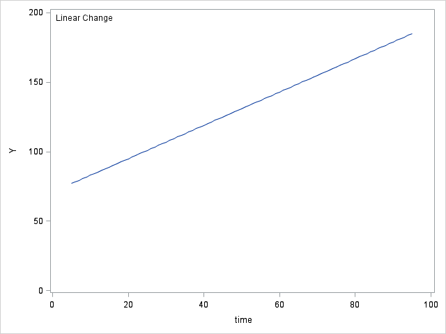
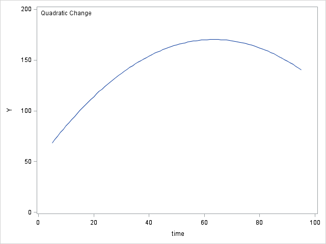
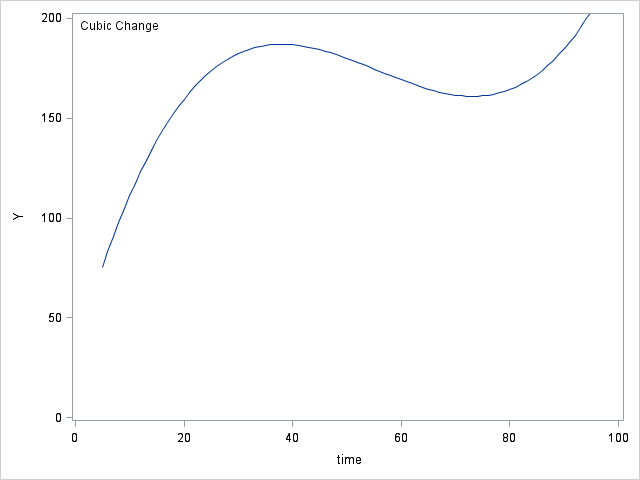
Figure 6.7 on page 218.
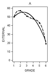
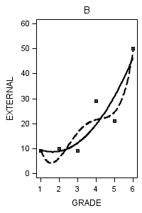
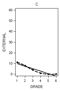
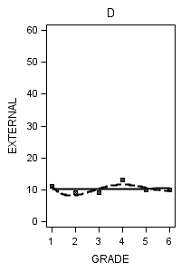
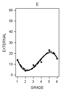
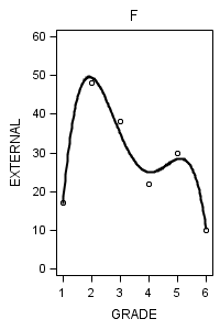
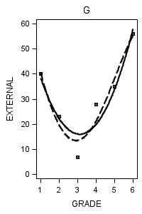
data figure6_7; set external_pp; if id = 1 then do; label = "A"; output; end; if id = 6 then do; label = "B"; output; end; if id = 11 then do; label = "C"; output; end; if id = 25 then do; label = "D"; output; end; if id = 34 then do; label = "E"; output; end; if id = 36 then do; label = "F"; output; end; if id = 40 then do; label = "G"; output; end; if id = 26 then do; label = "H"; output; end; run;
ods html style=journal3; ods graphics on /reset = all width=2in height=3in border=off;
proc sgplot data = figure6_7 (where = (label = "A")) noautolegend;
title "A";
yaxis min = 0 max = 60;
reg x = grade y = external / degree = 2 legendlabel = "Quadratic" lineattrs=(pattern = 1);
reg x = grade y = external / degree = 4 legendlabel = "Quartic" lineattrs=(pattern = 4);
run;
proc sgplot data = figure6_7 (where = (label = "B")) noautolegend;
title "B";
yaxis min = 0 max = 60;
reg x = grade y = external / degree = 2 legendlabel = "Quadratic" lineattrs=(pattern = 1);
reg x = grade y = external / degree = 4 legendlabel = "Quartic" lineattrs=(pattern = 4);
run;
proc sgplot data = figure6_7 (where = (label = "C")) noautolegend;
title "C";
yaxis min = 0 max = 60;
reg x = grade y = external / degree = 1 legendlabel = "linear" lineattrs=(pattern = 1);
reg x = grade y = external / degree = 4 legendlabel = "Quartic" lineattrs=(pattern = 4);
run;
proc sgplot data = figure6_7 (where = (label = "D")) noautolegend;
title "D";
yaxis min = 0 max = 60;
reg x = grade y = external / degree = 1 legendlabel = "linear" lineattrs=(pattern = 1);
reg x = grade y = external / degree = 4 legendlabel = "Quartic" lineattrs=(pattern = 4);
run;
proc sgplot data = figure6_7 (where = (label = "E")) noautolegend;
title "E";
yaxis min = 0 max = 60;
reg x = grade y = external / degree = 3 legendlabel = "Cubic" lineattrs=(pattern = 1);
reg x = grade y = external / degree = 4 legendlabel = "Quartic" lineattrs=(pattern = 4);
run;
proc sgplot data = figure6_7 (where = (label = "F")) noautolegend;
title "F";
yaxis min = 0 max = 60;
reg x = grade y = external / degree = 4 ;
run;
proc sgplot data = figure6_7 (where = (label = "G")) noautolegend;
title "G";
yaxis min = 0 max = 60;
reg x = grade y = external / degree = 2 legendlabel = "Quadratic" lineattrs=(pattern = 1);
reg x = grade y = external / degree = 4 legendlabel = "Quartic" lineattrs=(pattern = 4);
run;
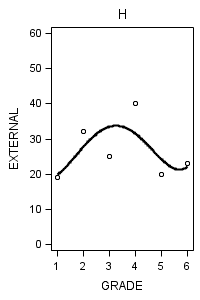
proc sgplot data = figure6_7 (where = (label = "H")) noautolegend;
title "H";
yaxis min = 0 max = 60;
reg x = grade y = external / degree = 4 ;
run;
To put them all together in a simpler way, we can also do the following.
ods graphics on /reset = all width = 6.5in height=5in border=off; title; proc sgpanel data = figure6_7; panelby label / columns = 4 spacing = 5 novarname; rowaxis min = 0 max = 60; reg x = grade y = external / degree = 1 legendlabel = "Linear" lineattrs=(pattern = 1); reg x = grade y = external / degree = 2 legendlabel = "Quadratic" lineattrs=(pattern = 4); reg x = grade y = external / degree = 3 legendlabel = "Cubic" lineattrs=(pattern = 1); reg x = grade y = external / degree = 4 legendlabel = "Quartic" lineattrs=(pattern = 4); run;
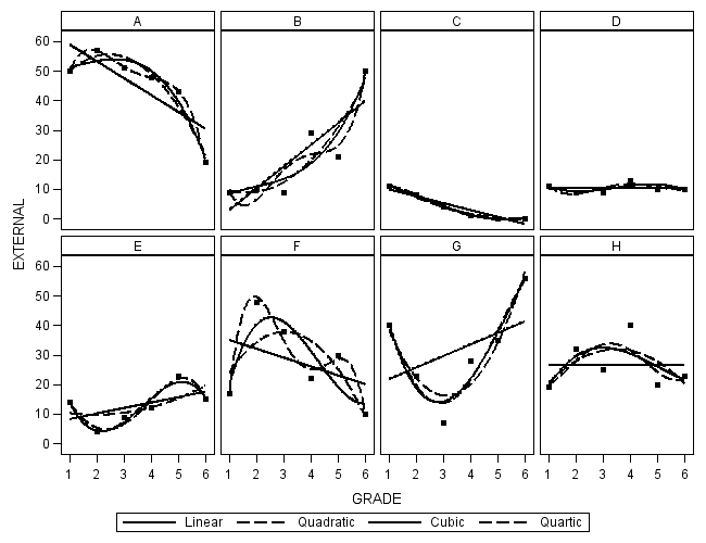
Table 6.5 on page 221.
title1 'Table 6.5: Alternative polynomial change trajectories for externalizing data'; proc mixed data = external_pp method=ml; title2 'Model A No Change'; class id; model external = / solution; random intercept / subject = id type=un;; run; proc mixed data = external_pp method = ml; title2 'Model B Linear Change'; class id; model external = time / solution; random intercept time / subject = id type=un;; run; proc mixed data = external_pp method = ml; title2 'Model C Quadratic Change'; class id; model external = time|time / solution; random intercept time|time / subject = id type=un; run; proc mixed data = external_pp method = ml; title2 'Model D Cubic Change'; class id; model external = time|time|time / solution; random intercept time|time|time / subject = id type=un; run;
Table 6.5: Alternative polynomial change trajectories for externalizing data
Model A No Change
The Mixed Procedure
Model Information
Data Set WORK.EXTERNAL_PP
Dependent Variable EXTERNAL
Covariance Structure Unstructured
Subject Effect ID
Estimation Method ML
Residual Variance Method Profile
Fixed Effects SE Method Model-Based
Degrees of Freedom Method Containment
Class Level Information
Class Levels Values
ID 45 1 2 3 4 5 6 7 8 9 10 11 12 13
14 15 16 17 18 19 20 21 22 23
24 25 26 27 28 29 30 31 32 33
34 35 36 37 38 39 40 41 42 43
44 45
Dimensions
Covariance Parameters 2
Columns in X 1
Columns in Z Per Subject 1
Subjects 45
Max Obs Per Subject 6
Number of Observations
Number of Observations Read 270
Number of Observations Used 270
Number of Observations Not Used 0
Iteration History
Iteration Evaluations -2 Log Like Criterion
0 1 2132.47877447
1 1 2010.25302132 0.00000000
Convergence criteria met.
 Covariance Parameter Estimates
Cov Parm     Subject    Estimate
UN(1,1) ID 87.4179
Residual 70.2030
Fit Statistics
-2 Log Likelihood 2010.3
AIC (smaller is better) 2016.3
AICC (smaller is better) 2016.3
BIC (smaller is better) 2021.7
Null Model Likelihood Ratio Test
DF Chi-Square Pr > ChiSq
1 122.23 <.0001
Solution for Fixed Effects
Standard
Effect Estimate Error DF t Value Pr > |t|
Intercept 12.9630 1.4841 44 8.73 <.0001
Model B Linear Change
The Mixed Procedure
Model Information
Data Set WORK.EXTERNAL_PP
Dependent Variable EXTERNAL
Covariance Structure Unstructured
Subject Effect ID
Estimation Method ML
Residual Variance Method Profile
Fixed Effects SE Method Model-Based
Degrees of Freedom Method Containment
Class Level Information
Class Levels Values
ID 45 1 2 3 4 5 6 7 8 9 10 11 12 13
14 15 16 17 18 19 20 21 22 23
24 25 26 27 28 29 30 31 32 33
34 35 36 37 38 39 40 41 42 43
44 45
Dimensions
Covariance Parameters 4
Columns in X 2
Columns in Z Per Subject 2
Subjects 45
Max Obs Per Subject 6
Number of Observations
Number of Observations Read 270
Number of Observations Used 270
Number of Observations Not Used 0
Iteration History
Iteration Evaluations -2 Log Like Criterion
0 1 2132.39329163
1 1 1991.74445476 0.00000000
Convergence criteria met.
 Covariance Parameter Estimates
Cov Parm     Subject    Estimate
UN(1,1) ID 123.52
UN(2,1) ID -12.5379
UN(2,2) ID 4.6929
Residual 53.7180
Fit Statistics
-2 Log Likelihood 1991.7
AIC (smaller is better) 2003.7
AICC (smaller is better) 2004.1
BIC (smaller is better) 2014.6
Null Model Likelihood Ratio Test
DF Chi-Square Pr > ChiSq
3 140.65 <.0001
Solution for Fixed Effects
Standard
Effect Estimate Error DF t Value Pr > |t|
Intercept 13.2899 1.8358 44 7.24 <.0001
TIME -0.1308 0.4153 44 -0.31 0.7543
Type 3 Tests of Fixed Effects
Num Den
Effect DF DF F Value Pr > F
TIME 1 44 0.10 0.7543
Model C Quadratic Change
The Mixed Procedure
Model Information
Data Set WORK.EXTERNAL_PP
Dependent Variable EXTERNAL
Covariance Structure Unstructured
Subject Effect ID
Estimation Method ML
Residual Variance Method Profile
Fixed Effects SE Method Model-Based
Degrees of Freedom Method Containment
Class Level Information
Class Levels Values
ID 45 1 2 3 4 5 6 7 8 9 10 11 12 13
14 15 16 17 18 19 20 21 22 23
24 25 26 27 28 29 30 31 32 33
34 35 36 37 38 39 40 41 42 43
44 45
Dimensions
Covariance Parameters 7
Columns in X 3
Columns in Z Per Subject 3
Subjects 45
Max Obs Per Subject 6
Number of Observations
Number of Observations Read 270
Number of Observations Used 270
Number of Observations Not Used 0
Iteration History
Iteration Evaluations -2 Log Like Criterion
0 1 2131.94936085
1 1 1975.83643546 0.00000000
Convergence criteria met.
Covariance Parameter Estimates
Cov Parm Subject Estimate
UN(1,1) ID 107.09
UN(2,1) ID -3.6906
UN(2,2) ID 24.6099
UN(3,1) ID -1.3617
UN(3,2) ID -4.9638
UN(3,3) ID 1.2157
Residual 41.9836
Fit Statistics
-2 Log Likelihood 1975.8
AIC (smaller is better) 1995.8
AICC (smaller is better) 1996.7
BIC (smaller is better) 2013.9
Null Model Likelihood Ratio Test
DF Chi-Square Pr > ChiSq
6 156.11 <.0001
Solution for Fixed Effects
Standard
Effect Estimate Error DF t Value Pr > |t|
Intercept 13.9698 1.7737 44 7.88 <.0001
TIME -1.1506 1.1068 44 -1.04 0.3042
TIME*TIME 0.2040 0.2280 44 0.89 0.3760
Type 3 Tests of Fixed Effects
Num Den
Effect DF DF F Value Pr > F
TIME 1 44 1.08 0.3042
TIME*TIME 1 44 0.80 0.3760
Model D Cubic Change
The Mixed Procedure
Model Information
Data Set WORK.EXTERNAL_PP
Dependent Variable EXTERNAL
Covariance Structure Unstructured
Subject Effect ID
Estimation Method ML
Residual Variance Method Profile
Fixed Effects SE Method Model-Based
Degrees of Freedom Method Containment
Class Level Information
Class Levels Values
ID 45 1 2 3 4 5 6 7 8 9 10 11 12 13
14 15 16 17 18 19 20 21 22 23
24 25 26 27 28 29 30 31 32 33
34 35 36 37 38 39 40 41 42 43
44 45
Dimensions
Covariance Parameters 11
Columns in X 4
Columns in Z Per Subject 4
Subjects 45
Max Obs Per Subject 6
Number of Observations
Number of Observations Read 270
Number of Observations Used 270
Number of Observations Not Used 0
Iteration History
Iteration Evaluations -2 Log Like Criterion
0 1 2131.88605549
1 2 1978.97160127 1669981.1326
2 2 1969.48069626 0.00720224
3 2 1967.43905341 0.00054013
4 1 1966.98742360 0.00003334
5 1 1966.96182113 0.00000016
6 1 1966.96170069 0.00000000
Convergence criteria met.
Covariance Parameter Estimates
Cov Parm Subject Estimate
UN(1,1) ID 126.93
UN(2,1) ID -53.6830
UN(2,2) ID 94.1321
UN(3,1) ID 23.6750
UN(3,2) ID -34.1029
UN(3,3) ID 12.4952
UN(4,1) ID -3.1578
UN(4,2) ID 3.1397
UN(4,3) ID -1.1091
UN(4,4) ID 0.09627
Residual 39.8305
Fit Statistics
-2 Log Likelihood 1967.0
AIC (smaller is better) 1997.0
AICC (smaller is better) 1998.9
BIC (smaller is better) 2024.1
Null Model Likelihood Ratio Test
DF Chi-Square Pr > ChiSq
10 164.92 <.0001
Solution for Fixed Effects
Standard
Effect Estimate Error DF t Value Pr > |t|
Intercept 13.7945 1.9159 44 7.20 <.0001
TIME -0.3501 2.3019 44 -0.15 0.8798
TIME*TIME -0.2343 1.0343 44 -0.23 0.8218
TIME*TIME*TIME 0.05844 0.1257 44 0.46 0.6443
Type 3 Tests of Fixed Effects
Num Den
Effect DF DF F Value Pr > F
TIME 1 44 0.02 0.8798
TIME*TIME 1 44 0.05 0.8218
TIME*TIME*TIME 1 44 0.22 0.6443
Figure 6.8 on page 227.
proc sgpanel data = foxngeese_pp (where = (id in(1, 4, 6, 7, 8, 11, 12, 15))) ;
  title "Figure 6.8 Empirical growth plots for 8 children";
  panelby id / columns = 4 rows = 2 spacing = 5;
  scatter x = game y = nmoves ;
run;
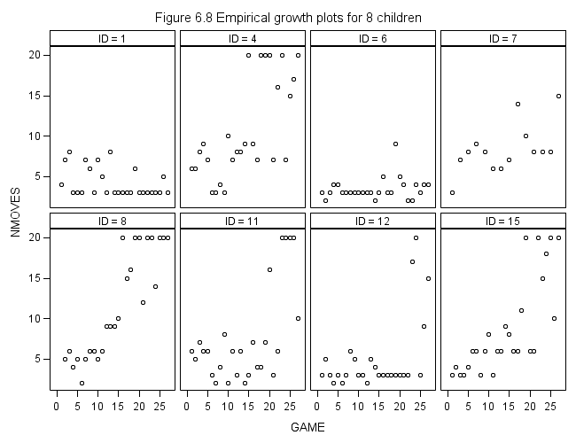
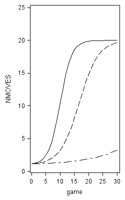
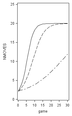
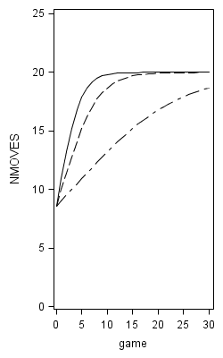
Figure 6.9 on page 229.
data fig6_9;
  do game = 0 to 30 ;
    y1 = 1 + 19/(1 + 150*exp(-.5*game));
	y2 = 1 + 19/(1 + 150*exp(-.3*game));
    y3 = 1 + 19/(1 + 150*exp(-.1*game));
    y4 = 1 + 19/(1 + 15*exp(-.5*game));
    y5 = 1 + 19/(1 + 15*exp(-.3*game));
    y6 = 1 + 19/(1 + 15*exp(-.1*game));
    y7 = 1 + 19/(1 + 1.50*exp(-.5*game));
    y8 = 1 + 19/(1 + 1.50*exp(-.3*game));
    y9 = 1 + 19/(1 + 1.50*exp(-.1*game));
    output;
  end;
run;
ods graphics on /reset = all width = 2.5in height=4in border=off;
title;
proc sgplot data = fig6_9 noautolegend;
  yaxis min = 0 max =25;
  label y1 = "NMOVES";
  series x = game y = y1;
  series x = game y = y2;
  series x = game y = y3;
run;

proc sgplot data = fig6_9 noautolegend;
  yaxis min = 0 max =25;
  label y4 = "NMOVES";
  series x = game y = y4;
  series x = game y = y5;
  series x = game y = y6;
run;
proc sgplot data = fig6_9 noautolegend;
  yaxis min = 0 max =25;
  label y7 = "NMOVES";
  series x = game y = y7;
  series x = game y = y8;
  series x = game y = y9;
run;
Table 6.6 on page 231. Notice, this model does not correspond to equation (6.8) in the book. Instead, it corresponds to the following equation:
Yij = 1 + 19/(1 + π0*exp(- (π1+u1)*Time – u0)) + εij
title1 'Table 6.6: Logistic change trajectories for Fox n Geese Data';
data foxngeese1;
  set 'c:\alda\foxngeese_pp';
  read=read-1.95625;
  readgame=read*game;
run;

proc nlmixed data=foxngeese1 maxiter=1000;
  title2 'Model A: Unconditional logistic growth trajectory';
  parms G00=12 G10=.1 s2e=20 s2u0=.3 cu10=0 s2u1=.01;
  num = 19;
  den = 1 + G00*(exp(-(G10*GAME +u0 +u1*GAME)));
  model NMOVES ~ normal(1+num/den,s2e);
  random u0 u1 ~ normal([0,0],[s2u0,cu10,s2u1]) subject=id;
run;

proc nlmixed data=foxngeese1 maxiter=1000;
  title2 'Model B: Effect of READing scores on 'intercept' and 'slope'';
  parms G00=12 G10=.12 G01=-.4 G11=.04 s2e=14 s2u0=.5 cu10=0 s2u1=.01;
  num = 19;
  den = 1 + G00*(exp(-(G01*READ + G10*GAME +G11*READGAME +u0 +u1*GAME)));
  model NMOVES ~ normal(1+num/den,s2e);
  random u0 u1 ~ normal([0,0],[s2u0,cu10,s2u1]) subject=id;
run;
Table 6.6: Logistic change trajectories for Fox n Geese Data
Model A: Unconditional logistic growth trajectory
The NLMIXED ProcedureSpecifications Data Set WORK.FOXNGEESE1 Dependent Variable NMOVES Distribution for Dependent Variable Normal Random Effects u0 u1 Distribution for Random Effects Normal Subject Variable ID Optimization Technique Dual Quasi-Newton Integration Method Adaptive Gaussian Quadrature
Dimensions Observations Used 445 Observations Not Used 0 Total Observations 445 Subjects 17 Max Obs Per Subject 27 Parameters 6 Quadrature Points 5Parameters G00 G10 s2e s2u0 cu10 s2u1 NegLogLike 12 0.1 20 0.3 0 0.01 1261.25
Iteration History
Iter Calls NegLogLike Diff MaxGrad Slope 1 7 1258.52475 2.725243 657.8958 -2406.51 2 11 1258.03268 0.492073 1419.048 -192.518 3 13 1256.09222 1.940463 1769.457 -20.6913 4 15 1255.48089 0.611323 2337.157 -100.908 5 16 1254.54565 0.935244 607.5571 -5.17012 6 20 1253.96624 0.579413 316.309 -0.58836 7 21 1253.12494 0.8413 494.2391 -0.34738 8 23 1248.9498 4.175134 230.3647 -0.5671 9 25 1247.93649 1.013312 398.5944 -4.26934 10 27 1247.58877 0.347722 383.4681 -0.36899 11 29 1247.36045 0.228322 413.4435 -0.17984 12 31 1246.70425 0.656196 502.2386 -0.29338 13 37 1242.64028 4.063972 265.338 -0.47028 14 39 1241.9899 0.650374 899.0315 -5.74098 15 40 1241.55511 0.434794 205.7158 -8.35368 16 41 1240.94052 0.614588 20.98148 -1.19379 17 45 1240.80525 0.135269 282.8497 -0.2504 18 46 1240.75395 0.051304 51.88217 -0.08082 19 47 1240.66772 0.086229 38.56674 -0.15795 20 48 1240.63714 0.030578 48.70844 -0.07439 21 50 1240.49786 0.13928 163.4847 -0.15154 22 54 1239.95757 0.540286 235.3687 -0.13449 23 56 1239.91523 0.042349 112.3383 -0.173 24 57 1239.89566 0.019565 98.87928 -0.10346 25 59 1239.88347 0.01219 8.84369 -0.02542 26 61 1239.88299 0.000483 5.588885 -0.00153 27 63 1239.88281 0.00018 2.483496 -0.00038 28 64 1239.88266 0.000145 4.155102 -0.00009 29 66 1239.88114 0.001527 13.31544 -0.00036 30 68 1239.85716 0.023973 3.172444 -0.0026 31 70 1239.85403 0.003134 0.283367 -0.0057 32 72 1239.8539 0.000134 0.052657 -0.00026 33 74 1239.8539 1.763E-7 0.006638 -3.62E-7
NOTE: GCONV convergence criterion satisfied.
Fit Statistics -2 Log Likelihood 2479.7 AIC (smaller is better) 2491.7 AICC (smaller is better) 2491.9 BIC (smaller is better) 2496.7Parameter Estimates
Standard Parameter Estimate Error DF t Value Pr > |t| Alpha Lower G00 12.9551 3.6330 15 3.57 0.0028 0.05 5.2115 G10 0.1227 0.02352 15 5.22 0.0001 0.05 0.07259 s2e 13.4005 0.9379 15 14.29 <.0001 0.05 11.4014 s2u0 0.6761 0.4551 15 1.49 0.1581 0.05 -0.2939 cu10 -0.05855 0.03553 15 -1.65 0.1202 0.05 -0.1343 s2u1 0.007239 0.003313 15 2.19 0.0452 0.05 0.000178
Parameter Estimates
Parameter Upper Gradient G00 20.6987 -6.66E-6 G10 0.1729 0.000886 s2e 15.3997 1.046E-6 s2u0 1.6461 0.000058 cu10 0.01719 0.000046 s2u1 0.01430 -0.00664
Table 6.6: Logistic change trajectories for Fox n Geese Data Model B: Effect of READing scores on intercept and slopeThe NLMIXED Procedure
Specifications Data Set WORK.FOXNGEESE1 Dependent Variable NMOVES Distribution for Dependent Variable Normal Random Effects u0 u1 Distribution for Random Effects Normal Subject Variable ID Optimization Technique Dual Quasi-Newton Integration Method Adaptive Gaussian Quadrature
Dimensions Observations Used 445 Observations Not Used 0 Total Observations 445 Subjects 17 Max Obs Per Subject 27 Parameters 8 Quadrature Points 5
Parameters
G00 G10 G01 G11 s2e s2u0 cu10 s2u1 12 0.12 -0.4 0.04 14 0.5 0 0.01
Parameters
NegLogLike
1246.43422
Iteration HistoryIter Calls NegLogLike Diff MaxGrad Slope 1 7 1243.63566 2.798559 567.8627 -2396.1 2 11 1243.14878 0.486877 1275.946 -193.445 3 13 1241.4908 1.657982 3419.608 -19.4135 4 15 1241.12233 0.368471 3858.482 -61.0749 5 17 1239.72337 1.398955 909.5793 -10.2729 6 19 1239.54041 0.182963 632.7479 -16.6481 7 20 1239.23789 0.302523 513.0341 -0.55705 8 22 1239.1108 0.127092 187.6112 -0.16517 9 24 1239.08713 0.02367 62.71314 -0.03245 10 26 1239.07617 0.010952 18.52108 -0.01113 11 28 1239.03017 0.046004 160.0849 -0.00684 12 29 1238.96737 0.062802 112.5344 -0.03578 13 31 1238.95343 0.013934 9.737014 -0.01902 14 32 1238.9492 0.004236 211.1171 -0.00856 15 34 1238.93233 0.016867 31.65528 -0.02366 16 36 1238.92435 0.00798 6.971984 -0.00681 17 38 1238.92418 0.000168 6.217619 -0.00014 18 40 1238.92159 0.002595 34.87699 -0.00016 19 41 1238.91823 0.003359 6.663299 -0.0034 20 43 1238.91664 0.001585 31.45648 -0.00097 21 45 1238.89623 0.020408 9.595661 -0.00183 22 47 1238.89535 0.000887 1.692847 -0.00155 23 49 1238.89534 6.399E-6 0.032296 -0.00001
NOTE: GCONV convergence criterion satisfied.
Fit Statistics -2 Log Likelihood 2477.8 AIC (smaller is better) 2493.8 AICC (smaller is better) 2494.1 BIC (smaller is better) 2500.5Parameter Estimates
Standard Parameter Estimate Error DF t Value Pr > |t| Alpha Lower G00 12.8840 3.4377 15 3.75 0.0019 0.05 5.5567 G10 0.1223 0.02193 15 5.58 <.0001 0.05 0.07558
Parameter Estimates
Parameter Upper Gradient G00 20.2114 0.000177 G10 0.1690 -0.0323
Parameter Estimates
Standard Parameter Estimate Error DF t Value Pr > |t| Alpha Lower G01 -0.3745 0.3359 15 -1.11 0.2825 0.05 -1.0906 G11 0.04049 0.02852 15 1.42 0.1761 0.05 -0.02029 s2e 13.4165 0.9399 15 14.27 <.0001 0.05 11.4131 s2u0 0.5610 0.4078 15 1.38 0.1891 0.05 -0.3082 cu10 -0.04685 0.03117 15 -1.50 0.1535 0.05 -0.1133 s2u1 0.006055 0.002893 15 2.09 0.0538 0.05 -0.00011
Parameter      Upper    Gradient
G01           0.3415    0.000707
G11           0.1013    0.009103
s2e          15.4200    0.000146
s2u0          1.4301    0.000789
cu10         0.01958    0.015416
s2u1         0.01222    0.024415
Figure 6.10 on page 232.
proc nlmixed data=foxngeese1 maxiter=1000;
  parms G00=12 G10=.1 s2e=20 s2u0=.3 cu10=0 s2u1=.01;
  num = 19;
  den = 1 + G00*(exp(-(G10*GAME +u0 +u1*GAME)));
  p = 1 + num/(1  + G00*exp(-(G10*GAME)));
  model NMOVES ~ normal(1+num/den,s2e);
  random u0 u1 ~ normal([0,0],[s2u0,cu10,s2u1]) subject=id;
  predict p out=modela;
run;

proc sort data = modela;
  by game;
run;
title "Model A";
proc sgplot data = modela;
  yaxis min = 0 max =25;
  series x = game y = pred;
run;

proc nlmixed data=foxngeese1 maxiter=1000;
  parms G00=12 G10=.12 G01=-.4 G11=.04 s2e=14 s2u0=.5 cu10=0 s2u1=.01;
  num = 19;
  den = 1 + G00*(exp(-(G01*READ + G10*GAME +G11*READGAME +u0 +u1*GAME)));
  plow = 1 + num/(1 + G00*exp(-(G01*(-1.58) + G10*GAME +G11*game*(-1.58))));
  phigh = 1 + num/(1 + G00*exp(-(G01*1.58 + G10*GAME +G11*GAME*1.58)));
  model NMOVES ~ normal(1+num/den,s2e);
  random u0 u1 ~ normal([0,0],[s2u0,cu10,s2u1]) subject=id;
  predict plow  out=modelb_low;
  predict phigh  out=modelb_high;
run;
data modelb;
  merge modelb_low (keep=id game pred rename = (pred=plow))
        modelb_high (keep=id game pred rename = (pred=phigh));
  by id;
run;

proc sort data = modelb;
  by game;
run;
title "Model B";
proc sgplot data = modelb noautolegend;
  yaxis min = 0 max =25;
  series x = game y = plow;
  series x = game y = phigh;
run;
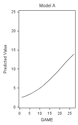
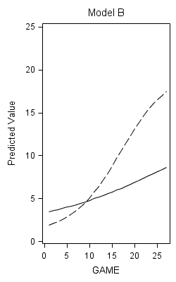
Figure 6.11 on page 235.
proc template;
define style newstyle;
	style GraphData1/
		Contrastcolor = light gray;
	style GraphData2/
		Contrastcolor = gray;
	style GraphData3/
		Contrastcolor = black;
end;
run;

ods html style=newstyle;

proc format library=mylib;
value fig 1 = 'Hyperbola'
          2 = 'Inverse Polynomial'
		  3 = 'Exponential'
		  4 = 'Negative Exponential';
run;

options fmtsearch = (mylib);

data hyperbola;
plot = 1;
do time = 1 to 10 by 0.01;
	pi = 0.01;
	y = 100 - 1/(pi*time);
	output;
end;
do time = .5 to 10 by 0.01;
	pi = 0.02;
	y = 100 - 1/(pi*time);
	output;
end;
do time = .1 to 10 by 0.01;
	pi = 0.1;
	y = 100 - 1/(pi*time);
	output;
end;
run;

data invpoly;
plot = 2;
do time = .5204 to 10 by 0.01;
	pi = -0.0015;
	y = 100 - 1/(0.02*time + pi*time*time);
	output;
end;
do time = .5 to 10 by 0.01;
	pi = 0;
	y = 100 - 1/(0.02*time + pi*time*time);
	output;
end;
do time = .39 to 10 by 0.01;
	pi = 0.015;
	y = 100 - 1/(0.02*time + pi*time*time);
	output;
end;

data exponential;
plot = 3;
do time = 0 to 10 by 0.01;
	pi = 0.1;
	y = 5*exp(pi*time);
	output;
	pi = 0.2;
	y = 5*exp(pi*time);
	output;
	pi = 0.3;
	y = 5*exp(pi*time);
	output;
end;
run;

data negexponential;
plot = 4;
do time = 0 to 10 by 0.01;
	pi = 0.1;
	y = 100-(100-20)*exp(-pi*time);
	output;
	pi = 0.2;
	y = 100-(100-20)*exp(-pi*time);
	output;
	pi = 0.3;
	y = 100-(100-20)*exp(-pi*time);
	output;
end;
run;

data plotdata;
set hyperbola invpoly exponential negexponential;
format plot fig.;
run;

proc sgpanel data = plotdata noautolegend;
panelby plot;
series x = time y = y / group = pi;
refline 100 / lineattrs=(pattern=4);
run;
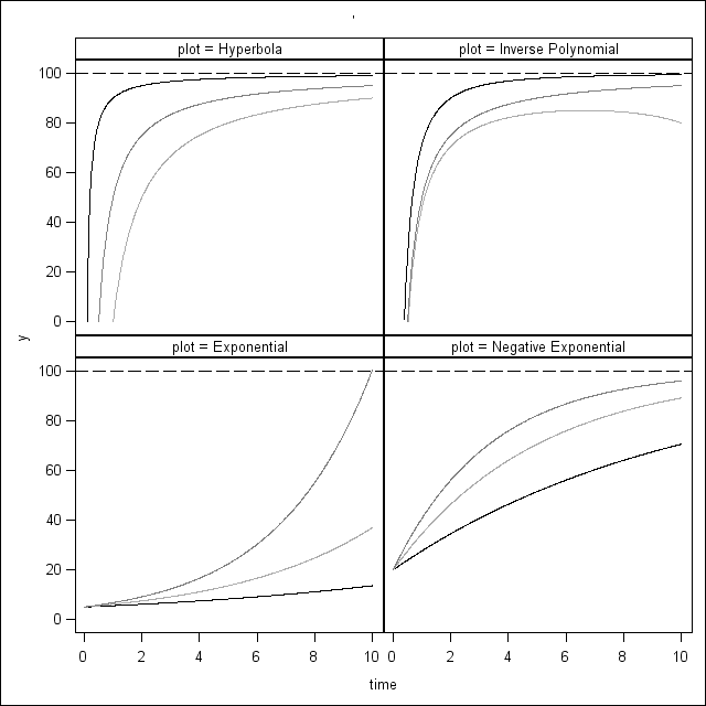
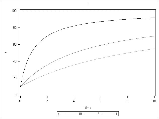
Figure 6.12 on page 242.
data thurstone;
do time = 0 to 10 by 0.01;
	pi = 10;
	y = 10 + ((100 - 10)*time)/(pi + time);
	output;
	pi = 5;
	y = 10 + ((100 - 10)*time)/(pi + time);
	output;
	pi = 1;
	y = 10 + ((100 - 10)*time)/(pi + time);
	output;
end;
run;

proc sgplot data = thurstone;
series x = time y = y / group = pi;
yaxis min = 0 max = 100;
refline 100 / lineattrs = (pattern=4);
run;
