5.2.2 The Hosmer-Lemeshow Tests
page 150 Table 5.1 Observed (obs) and estimated expected (exp) frequencies within each decile of risk, defined by fitted value (prob.) for dfree = 1 and dfree = 0 using the fitted logistic regression model in Table 4.9.
NOTE: Pursuant to the text on page 151 this table cannot be replicated in SAS. You can use Stata to obtain these values.
5.2.3 Classification tables
page 157 Table 5.2 Classification table based on the logistic regression model in Table 4.9 using a cutpoint of 0.5.
NOTE: We have bolded the relevant output.
data uis51;
  set 'd:hosmerdatauis';
  ndrgfp1 = ((ndrugtx+1)/10)**(-1);
  ndrgfp2 = ndrgfp1*log((ndrugtx+1)/10);
  agendrgfp1 = age*ndrgfp1;
  racesite = race*site;
run;
proc logistic data=uis51 desc;
  model dfree = age ndrgfp1 ndrgfp2 ivhx2 ivhx3 race treat site agendrgfp1 racesite
  / details ctable lackfit pprob = .5;
run;

The LOGISTIC Procedure

              Model Information

Data Set                      WORK.UIS51
Response Variable             DFREE
Number of Response Levels     2
Number of Observations        575
Link Function                 Logit
Optimization Technique        Fisher's scoring

          Response Profile

 Ordered                      Total
   Value        DFREE     Frequency
       1            1           147
       2            0           428

                    Model Convergence Status
         Convergence criterion (GCONV=1E-8) satisfied.

         Model Fit Statistics

                              Intercept
               Intercept         and
Criterion        Only        Covariates

AIC              655.729        619.963
SC               660.083        667.861
-2 Log L         653.729        597.963

        Testing Global Null Hypothesis: BETA=0

Test                 Chi-Square       DF     Pr > ChiSq

Likelihood Ratio        55.7660       10         <.0001
Score                   52.0723       10         <.0001
Wald                    47.2784       10         <.0001

The LOGISTIC Procedure

              Analysis of Maximum Likelihood Estimates

                                Standard
Parameter     DF    Estimate       Error    Chi-Square    Pr > ChiSq

Intercept      1     -6.8429      1.2193       31.4989        <.0001
AGE            1      0.1166      0.0289       16.3137        <.0001
ndrgfp1        1      1.6687      0.4071       16.8000        <.0001
ndrgfp2        1      0.4336      0.1169       13.7585        0.0002
IVHX2          1     -0.6346      0.2987        4.5134        0.0336
IVHX3          1     -0.7049      0.2616        7.2623        0.0070
RACE           1      0.6841      0.2641        6.7074        0.0096
TREAT          1      0.4349      0.2038        4.5559        0.0328
SITE           1      0.5162      0.2549        4.1013        0.0429
agendrgfp1     1     -0.0153     0.00603        6.4177        0.0113
racesite       1     -1.4294      0.5298        7.2799        0.0070

             Odds Ratio Estimates

                 Point          95% Wald
Effect        Estimate      Confidence Limits

AGE              1.124       1.062       1.189
ndrgfp1          5.306       2.389      11.784
ndrgfp2          1.543       1.227       1.940
IVHX2            0.530       0.295       0.952
IVHX3            0.494       0.296       0.825
RACE             1.982       1.181       3.326
TREAT            1.545       1.036       2.303
SITE             1.676       1.017       2.761
agendrgfp1       0.985       0.973       0.997
racesite         0.239       0.085       0.676

Association of Predicted Probabilities and Observed Responses

Percent Concordant     69.7    Somers' D    0.398
Percent Discordant     29.9    Gamma        0.399
Percent Tied            0.4    Tau-a        0.152
Pairs                 62916    c            0.699

The LOGISTIC Procedure

             Partition for the Hosmer and Lemeshow Test

                              DFREE = 1               DFREE = 0
   Group       Total    Observed    Expected    Observed    Expected

       1          58           4        4.10          54       53.90
       2          59           6        6.48          53       52.52
       3          59           7        8.78          52       50.22
       4          60          12       11.14          48       48.86
       5          60          16       13.35          44       46.65
       6          58          14       15.14          44       42.86
       7          58          19       17.92          39       40.08
       8          58          23       20.63          35       37.37
       9          58          21       24.79          37       33.21
      10          47          25       24.67          22       22.33

Hosmer and Lemeshow Goodness-of-Fit Test

Chi-Square       DF     Pr > ChiSq

    2.8735        8         0.9420

                          Classification Table

          Correct      Incorrect                Percentages
 Prob          Non-          Non-           Sensi-  Speci-  False  False
Level  Event  Event  Event  Event  Correct  tivity  ficity   POS    NEG

0.500     13    414     14    134     74.3     8.8    96.7   51.9   24.5
page 159 Table 5.3 Classification table based on the logistic regression model in Table 4.9 using a cutpoint of 0.5, but all probabilities pi-hat < 0.50 are replaced with pi-hat = 0.05 and all probabilities pi-hat >= 0.50 are replaced with pi-hat = 0.95.
NOTE: We were unable to reproduce this table. page 160 Table 5.4 Classification table based on the logistic regression model in Table 4.9 using a cutpoint of 0.5, but all probabilities pi-hat < 0.50 are replaced with pi-hat = 0.45 and all probabilities pi-hat >= 0.50 are replaced with pi-hat = 0.55.
NOTE: We were unable to reproduce this table.
5.2.4 Area under the ROC curve
page 161 Table 5.5 Classification table based on the logistic regression model in Table 4.9 using a cutpoint of 0.6.
proc logistic data=uis51 desc;
  model dfree = age ndrgfp1 ndrgfp2 ivhx2 ivhx3 race treat site agendrgfp1 racesite
  / details lackfit ctable pprob = .6;
run;

The LOGISTIC Procedure

              Model Information

Data Set                      WORK.UIS51
Response Variable             DFREE
Number of Response Levels     2
Number of Observations        575
Link Function                 Logit
Optimization Technique        Fisher's scoring

          Response Profile

 Ordered                      Total
   Value        DFREE     Frequency

       1            1           147
       2            0           428

                    Model Convergence Status

         Convergence criterion (GCONV=1E-8) satisfied.

         Model Fit Statistics

                              Intercept
               Intercept         and
Criterion        Only        Covariates

AIC              655.729        619.963
SC               660.083        667.861
-2 Log L         653.729        597.963

        Testing Global Null Hypothesis: BETA=0

Test                 Chi-Square       DF     Pr > ChiSq

Likelihood Ratio        55.7660       10         <.0001
Score                   52.0723       10         <.0001
Wald                    47.2784       10         <.0001

The LOGISTIC Procedure

              Analysis of Maximum Likelihood Estimates

                                Standard
Parameter     DF    Estimate       Error    Chi-Square    Pr > ChiSq

Intercept      1     -6.8429      1.2193       31.4989        <.0001
AGE            1      0.1166      0.0289       16.3137        <.0001
ndrgfp1        1      1.6687      0.4071       16.8000        <.0001
ndrgfp2        1      0.4336      0.1169       13.7585        0.0002
IVHX2          1     -0.6346      0.2987        4.5134        0.0336
IVHX3          1     -0.7049      0.2616        7.2623        0.0070
RACE           1      0.6841      0.2641        6.7074        0.0096
TREAT          1      0.4349      0.2038        4.5559        0.0328
SITE           1      0.5162      0.2549        4.1013        0.0429
agendrgfp1     1     -0.0153     0.00603        6.4177        0.0113
racesite       1     -1.4294      0.5298        7.2799        0.0070

             Odds Ratio Estimates

                 Point          95% Wald
Effect        Estimate      Confidence Limits

AGE              1.124       1.062       1.189
ndrgfp1          5.306       2.389      11.784
ndrgfp2          1.543       1.227       1.940
IVHX2            0.530       0.295       0.952
IVHX3            0.494       0.296       0.825
RACE             1.982       1.181       3.326
TREAT            1.545       1.036       2.303
SITE             1.676       1.017       2.761
agendrgfp1       0.985       0.973       0.997
racesite         0.239       0.085       0.676

Association of Predicted Probabilities and Observed Responses

Percent Concordant     69.7    Somers' D    0.398
Percent Discordant     29.9    Gamma        0.399
Percent Tied            0.4    Tau-a        0.152
Pairs                 62916    c            0.699

The LOGISTIC Procedure

             Partition for the Hosmer and Lemeshow Test

                              DFREE = 1               DFREE = 0
   Group       Total    Observed    Expected    Observed    Expected

       1          58           4        4.10          54       53.90
       2          59           6        6.48          53       52.52
       3          59           7        8.78          52       50.22
       4          60          12       11.14          48       48.86
       5          60          16       13.35          44       46.65
       6          58          14       15.14          44       42.86
       7          58          19       17.92          39       40.08
       8          58          23       20.63          35       37.37
       9          58          21       24.79          37       33.21
      10          47          25       24.67          22       22.33

Hosmer and Lemeshow Goodness-of-Fit Test

Chi-Square       DF     Pr > ChiSq

    2.8735        8         0.9420

                          Classification Table

          Correct      Incorrect                Percentages
 Prob          Non-          Non-           Sensi-  Speci-  False  False
Level  Event  Event  Event  Event  Correct  tivity  ficity   POS    NEG

0.600  3      428    0      144     75.0     2.0    100.0    0.0   25.2
page 161 Table 5.6 Summary of sensitivity, specificity, and 1-specificity for classification tables based on the logistic regression model in Table 4.9 using a cutpoint of 0.05 to 0.60 in increments of 0.05.
proc logistic data=uis51 desc;
  model dfree = age ndrgfp1 ndrgfp2 ivhx2 ivhx3 race treat site agendrgfp1 racesite
  / ctable pprob = (.05 to .6 by .05);
run;

The LOGISTIC Procedure

              Model Information

Data Set                      WORK.UIS51
Response Variable             DFREE
Number of Response Levels     2
Number of Observations        575
Link Function                 Logit
Optimization Technique        Fisher's scoring

          Response Profile

 Ordered                      Total
   Value        DFREE     Frequency

       1            1           147
       2            0           428

                   Model Convergence Status

         Convergence criterion (GCONV=1E-8) satisfied.

         Model Fit Statistics

                              Intercept
               Intercept         and
Criterion        Only        Covariates

AIC              655.729        619.963
SC               660.083        667.861
-2 Log L         653.729        597.963

        Testing Global Null Hypothesis: BETA=0

Test                 Chi-Square       DF     Pr > ChiSq

Likelihood Ratio        55.7660       10         <.0001
Score                   52.0723       10         <.0001
Wald                    47.2784       10         <.0001

The LOGISTIC Procedure

              Analysis of Maximum Likelihood Estimates

                                Standard
Parameter     DF    Estimate       Error    Chi-Square    Pr > ChiSq

Intercept      1     -6.8429      1.2193       31.4989        <.0001
AGE            1      0.1166      0.0289       16.3137        <.0001
ndrgfp1        1      1.6687      0.4071       16.8000        <.0001
ndrgfp2        1      0.4336      0.1169       13.7585        0.0002
IVHX2          1     -0.6346      0.2987        4.5134        0.0336
IVHX3          1     -0.7049      0.2616        7.2623        0.0070
RACE           1      0.6841      0.2641        6.7074        0.0096
TREAT          1      0.4349      0.2038        4.5559        0.0328
SITE           1      0.5162      0.2549        4.1013        0.0429
agendrgfp1     1     -0.0153     0.00603        6.4177        0.0113
racesite       1     -1.4294      0.5298        7.2799        0.0070

             Odds Ratio Estimates

                 Point          95% Wald
Effect        Estimate      Confidence Limits

AGE              1.124       1.062       1.189
ndrgfp1          5.306       2.389      11.784
ndrgfp2          1.543       1.227       1.940
IVHX2            0.530       0.295       0.952
IVHX3            0.494       0.296       0.825
RACE             1.982       1.181       3.326
TREAT            1.545       1.036       2.303
SITE             1.676       1.017       2.761
agendrgfp1       0.985       0.973       0.997
racesite         0.239       0.085       0.676

Association of Predicted Probabilities and Observed Responses

Percent Concordant     69.7    Somers' D    0.398
Percent Discordant     29.9    Gamma        0.399
Percent Tied            0.4    Tau-a        0.152
Pairs                 62916    c            0.699

                          Classification Table

          Correct      Incorrect                Percentages
 Prob          Non-          Non-           Sensi-  Speci-  False  False
Level  Event  Event  Event  Event  Correct  tivity  ficity   POS    NEG

0.050    146     10    418      1     27.1   99.3     2.3   74.1    9.1
0.100    140     65    363      7     35.7   95.2    15.2   72.2    9.7
0.150    130    134    294     17     45.9   88.4    31.3   69.3   11.3

The LOGISTIC Procedure

                          Classification Table

          Correct      Incorrect                Percentages
 Prob          Non-          Non-           Sensi-  Speci-  False  False
Level  Event  Event  Event  Event  Correct  tivity  ficity   POS    NEG

0.200    113    191    237     34     52.9   76.9    44.6   67.7   15.1
0.250     95    255    173     52     60.9   64.6    59.6   64.6   16.9
0.300     77    302    126     70     65.9   52.4    70.6   62.1   18.8
0.350     53    343     85     94     68.9   36.1    80.1   61.6   21.5
0.400     34    370     58    113     70.3   23.1    86.4   63.0   23.4
0.450     27    391     37    120     72.7   18.4    91.4   57.8   23.5
0.500     13    414     14    134     74.3    8.8    96.7   51.9   24.5
0.550      7    425      3    140     75.1    4.8    99.3   30.0   24.8
0.600      3    428      0    144     75.0    2.0    100.0    0.0   25.2
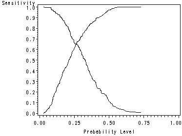
page 162 Figure 5.1 Plot of sensitivity and specificity versus all possible cutpoints in the UIS.
proc logistic data=uis51 desc;
  model dfree = age ndrgfp1 ndrgfp2 ivhx2 ivhx3 race treat site agendrgfp1 racesite
  / outroc=roc1;
run;
data roc2;
  set roc1;
  spec = 1-_1mspec_;
run;
symbol1 i=join v=none ;
proc gplot data=roc2;
  plot _sensit_*_PROB_=1 spec*_PROB_=1 / overlay haxis=0 to 1 by .25 vaxis=0 to 1 by .1 ;
run;
quit;

The LOGISTIC Procedure

              Model Information

Data Set                      WORK.UIS51
Response Variable             DFREE
Number of Response Levels     2
Number of Observations        575
Link Function                 Logit
Optimization Technique        Fisher's scoring

          Response Profile

 Ordered                      Total
   Value        DFREE     Frequency

       1            1           147
       2            0           428

                    Model Convergence Status

         Convergence criterion (GCONV=1E-8) satisfied.

         Model Fit Statistics

                              Intercept
               Intercept         and
Criterion        Only        Covariates

AIC              655.729        619.963
SC               660.083        667.861
-2 Log L         653.729        597.963

       Testing Global Null Hypothesis: BETA=0

Test                 Chi-Square       DF     Pr > ChiSq

Likelihood Ratio        55.7660       10         <.0001
Score                   52.0723       10         <.0001
Wald                    47.2784       10         <.0001

The LOGISTIC Procedure

              Analysis of Maximum Likelihood Estimates

                                Standard
Parameter     DF    Estimate       Error    Chi-Square    Pr > ChiSq

Intercept      1     -6.8429      1.2193       31.4989        <.0001
AGE            1      0.1166      0.0289       16.3137        <.0001
ndrgfp1        1      1.6687      0.4071       16.8000        <.0001
ndrgfp2        1      0.4336      0.1169       13.7585        0.0002
IVHX2          1     -0.6346      0.2987        4.5134        0.0336
IVHX3          1     -0.7049      0.2616        7.2623        0.0070
RACE           1      0.6841      0.2641        6.7074        0.0096
TREAT          1      0.4349      0.2038        4.5559        0.0328
SITE           1      0.5162      0.2549        4.1013        0.0429
agendrgfp1     1     -0.0153     0.00603        6.4177        0.0113
racesite       1     -1.4294      0.5298        7.2799        0.0070

             Odds Ratio Estimates

                 Point          95% Wald
Effect        Estimate      Confidence Limits

AGE              1.124       1.062       1.189
ndrgfp1          5.306       2.389      11.784
ndrgfp2          1.543       1.227       1.940
IVHX2            0.530       0.295       0.952
IVHX3            0.494       0.296       0.825
RACE             1.982       1.181       3.326
TREAT            1.545       1.036       2.303
SITE             1.676       1.017       2.761
agendrgfp1       0.985       0.973       0.997
racesite         0.239       0.085       0.676

Association of Predicted Probabilities and Observed Responses

Percent Concordant     69.7    Somers' D    0.398
Percent Discordant     29.9    Gamma        0.399
Percent Tied            0.4    Tau-a        0.152
Pairs                 62916    c            0.699
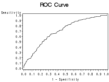
page 163 Figure 5.2 Plot of sensitivity versus 1-specificity for all possible cutpoints in the UIS. The resulting curve is called a ROC curve.
symbol1 i=join v=none ;
proc gplot data=roc1;
  title 'ROC Curve';
  plot _sensit_*_1mspec_=1 / vaxis=0 to 1 by .1 ;
run;
quit;
title;
5.3 Logistic regression diagnostics
page 171 Figure 5.3 Plot of leverage (h) versus the estimated logistic probability (pi-hat) for a hypothetical univariable logistic regression model.
NOTE: We cannot recreate this figure because we do have the hypothetical data that were used.
page 172 Figure 5.4 Plot of the distance portion of leverage (b) versus the estimated logistic probability (pi-hat) for a hypothetical univariable logistic regression model.
NOTE: We cannot recreate this figure because we do have the hypothetical data that were used.
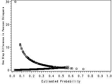
page 177 Figure 5.5 Plot of delta-x-square versus the estimated probability from the fitted model in Table 4.9, UIS J = 521 covariate patterns.
NOTE: This graph looks slightly different than the one in the book because SAS and Stata use different methods of handling covariate patterns. The graphs in the text were made using Stata.
proc logistic data=uis51 desc;
  model dfree = age ndrgfp1 ndrgfp2 ivhx2 ivhx3 race treat site agendrgfp1 racesite / aggregate scale = 1;
  output out=uis52 p=estprob DIFCHISQ=deltachi DIFDEV=deltad c=deltabeta;
run;
symbol1 i=none v=circle ;
axis1 order=(0 to 1 by .1) ;
axis2 label=(angle=90 color=black height=0.75);
proc gplot data=uis52;
  plot deltachi*estprob=1 / haxis=axis1 vaxis=axis2 ;
run;
quit;

The LOGISTIC Procedure

              Model Information

Data Set                      WORK.UIS51
Response Variable             DFREE
Number of Response Levels     2
Number of Observations        575
Link Function                 Logit
Optimization Technique        Fisher's scoring

          Response Profile

 Ordered                      Total
   Value        DFREE     Frequency

       1            1           147
       2            0           428

                    Model Convergence Status

         Convergence criterion (GCONV=1E-8) satisfied.

       Deviance and Pearson Goodness-of-Fit Statistics

Criterion        DF          Value     Value/DF     Pr > ChiSq

Deviance        510       530.7412       1.0407         0.2541
Pearson         510       511.7467       1.0034         0.4699

Number of unique profiles: 521

NOTE: The covariance matrix has been multiplied by the heterogeneity factor (square of SCALE=1)
      1.

         Model Fit Statistics

                              Intercept
               Intercept         and
Criterion        Only        Covariates

AIC              655.729        619.963
SC               660.083        667.861
-2 Log L         653.729        597.963

The LOGISTIC Procedure

        Testing Global Null Hypothesis: BETA=0

Test                 Chi-Square       DF     Pr > ChiSq

Likelihood Ratio        55.7660       10         <.0001
Score                   52.0723       10         <.0001
Wald                    47.2784       10         <.0001

              Analysis of Maximum Likelihood Estimates

                                Standard
Parameter     DF    Estimate       Error    Chi-Square    Pr > ChiSq

Intercept      1     -6.8429      1.2193       31.4989        <.0001
AGE            1      0.1166      0.0289       16.3137        <.0001
ndrgfp1        1      1.6687      0.4071       16.8000        <.0001
ndrgfp2        1      0.4336      0.1169       13.7585        0.0002
IVHX2          1     -0.6346      0.2987        4.5134        0.0336
IVHX3          1     -0.7049      0.2616        7.2623        0.0070
RACE           1      0.6841      0.2641        6.7074        0.0096
TREAT          1      0.4349      0.2038        4.5559        0.0328
SITE           1      0.5162      0.2549        4.1013        0.0429
agendrgfp1     1     -0.0153     0.00603        6.4177        0.0113
racesite       1     -1.4294      0.5298        7.2799        0.0070

            Odds Ratio Estimates

                 Point          95% Wald
Effect        Estimate      Confidence Limits

AGE              1.124       1.062       1.189
ndrgfp1          5.306       2.389      11.784
ndrgfp2          1.543       1.227       1.940
IVHX2            0.530       0.295       0.952
IVHX3            0.494       0.296       0.825
RACE             1.982       1.181       3.326
TREAT            1.545       1.036       2.303
SITE             1.676       1.017       2.761
agendrgfp1       0.985       0.973       0.997
racesite         0.239       0.085       0.676

Association of Predicted Probabilities and Observed Responses

Percent Concordant     69.7    Somers' D    0.398
Percent Discordant     29.9    Gamma        0.399
Percent Tied            0.4    Tau-a        0.152
Pairs                 62916    c            0.699
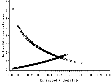
page 178 Figure 5.6 Plot of delta-D versus the estimated probability from the fitted model in Table 4.9, UIS J = 521 covariate patterns.
NOTE: This graph looks slightly different than the one in the book because SAS and Stata use different methods of handling covariate patterns. The graphs in the text were made using Stata.
symbol1 i=none v=circle ;
axis1 order=(0 to 1 by .1) ;
axis2 label=(angle=90 color=black height=0.75);
proc gplot data=uis52;
  plot deltad*estprob=1 / haxis=axis1 vaxis=axis2;
run;
quit;
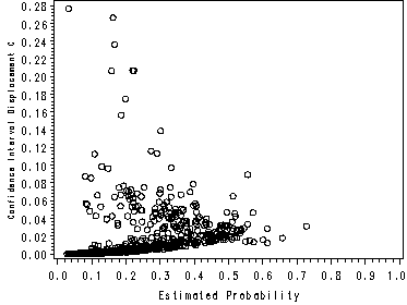
page 179 Figure 5.7 Plot of delta-beta-hat versus the estimated probability from the fitted model in Table 4.9, UIS J = 521 covariate patterns.
NOTE: This graph looks slightly different than the one in the book because SAS and Stata use different methods of handling covariate patterns. The graphs in the text were made using Stata.
symbol1 i=none v=circle ;
axis1 order=(0 to 1 by .1) ;
axis2 label=(angle=90 color=black height=0.75);
proc gplot data=uis52;
  plot deltabeta*estprob=1 / haxis=axis1 vaxis=axis2;
run;
quit;
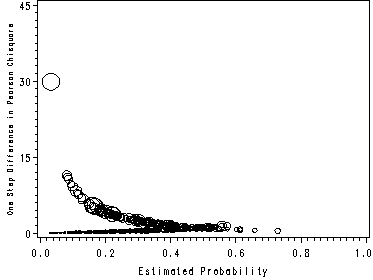
page 180 Figure 5.8 Plot of delta-chi-square versus the probability from the fitted model in Table 4.9 with size of the plotting symbol proportional to delta-beta-hat, UIS J = 521 covariate patterns.
NOTE: This graph looks slightly different than the one in the book because SAS and Stata use different methods of handling covariate patterns. The graphs in the text were made using Stata.
filename outgraph 'd:https://stats.idre.ucla.edu/wp-content/uploads/2016/02/hlch5sas6.gif';
goptions gsfname=outgraph dev=gif373;
symbol1 color=black interpol=r value=circle height=1;
axis1 order=(0 to 45 by 15) label=(angle=90 color=black height=0.75);
axis2 order=(0 to 1 by .2);
proc gplot data=uis52;
 bubble deltachi*estprob=deltabeta / bsize=20 haxis=axis2 vaxis=axis1;
run;
quit;
page 182 Table 5.8 Covariate values, observed outcome (yj), number (mj), estimated logistic probability (pi-hat), and the value of the four diagnostic statistics delta-beta-hat, delta-x-square, and leverage (h) for the four most extreme covariate patterns (P#).
NOTE: The following must be done to reproduce the covariate patterns as shown in the text, because SAS and Stata handle covariate patterns differently.
proc sort data=uis51 out=uis51sort nodupkey; by age ndrgfp1 ndrgfp2 ivhx2 ivhx3 race treat site agendrgfp1 racesite; run; proc sort data=uis51 out=uis51sorta; by age ndrgfp1 ndrgfp2 ivhx2 ivhx3 race treat site agendrgfp1 racesite; run; data uis53; set uis51sort; covpat=_n_; run; data uis54; merge uis51sorta uis53; by age ndrgfp1 ndrgfp2 ivhx2 ivhx3 race treat site agendrgfp1 racesite; run; proc logistic data=uis54 desc; model dfree = age ndrgfp1 ndrgfp2 ivhx2 ivhx3 race treat site agendrgfp1 racesite / aggregate scale = 1; output out=uis55 p=estprob DIFCHISQ=deltachi DIFDEV=deltad c=deltabeta h=lev; run; proc print data=uis55 noobs; var covpat age ndrugtx ivhx race treat site dfree estprob deltabeta deltachi deltad lev; where covpat=31 or covpat=477 or covpat=105 or covpat=468; run;The LOGISTIC Procedure
Model Information
Data Set WORK.UIS54 Response Variable DFREE Number of Response Levels 2 Number of Observations 575 Link Function Logit Optimization Technique Fisher's scoring
Response Profile
Ordered Total Value DFREE Frequency
1 1 147 2 0 428
Model Convergence Status
Convergence criterion (GCONV=1E-8) satisfied.
Deviance and Pearson Goodness-of-Fit Statistics
Criterion DF Value Value/DF Pr > ChiSq
Deviance 510 530.7412 1.0407 0.2541 Pearson 510 511.7467 1.0034 0.4699
Number of unique profiles: 521
NOTE: The covariance matrix has been multiplied by the heterogeneity factor (square of SCALE=1) 1.
Model Fit Statistics
Intercept Intercept and Criterion Only Covariates
AIC 655.729 619.963 SC 660.083 667.861 -2 Log L 653.729 597.963
The LOGISTIC Procedure
Testing Global Null Hypothesis: BETA=0
Test Chi-Square DF Pr > ChiSq
Likelihood Ratio 55.7660 10 <.0001 Score 52.0723 10 <.0001 Wald 47.2784 10 <.0001
Analysis of Maximum Likelihood Estimates
Standard Parameter DF Estimate Error Chi-Square Pr > ChiSq
Intercept 1 -6.8429 1.2193 31.4989 <.0001 AGE 1 0.1166 0.0289 16.3137 <.0001 ndrgfp1 1 1.6687 0.4071 16.8000 <.0001 ndrgfp2 1 0.4336 0.1169 13.7585 0.0002 IVHX2 1 -0.6346 0.2987 4.5134 0.0336 IVHX3 1 -0.7049 0.2616 7.2623 0.0070 RACE 1 0.6841 0.2641 6.7074 0.0096 TREAT 1 0.4349 0.2038 4.5559 0.0328 SITE 1 0.5162 0.2549 4.1013 0.0429 agendrgfp1 1 -0.0153 0.00603 6.4177 0.0113 racesite 1 -1.4294 0.5298 7.2799 0.0070
Odds Ratio Estimates
Point 95% Wald Effect Estimate Confidence Limits
AGE 1.124 1.062 1.189 ndrgfp1 5.306 2.389 11.784 ndrgfp2 1.543 1.227 1.940 IVHX2 0.530 0.295 0.952 IVHX3 0.494 0.296 0.825 RACE 1.982 1.181 3.326 TREAT 1.545 1.036 2.303 SITE 1.676 1.017 2.761 agendrgfp1 0.985 0.973 0.997 racesite 0.239 0.085 0.676
Association of Predicted Probabilities and Observed Responses
Percent Concordant 69.7 Somers' D 0.398 Percent Discordant 29.9 Gamma 0.399 Percent Tied 0.4 Tau-a 0.152 Pairs 62916 c 0.699
covpat AGE NDRUGTX IVHX RACE TREAT SITE DFREE estprob deltabeta deltachi  deltad    lev

   31   24    20     2    0    0     1    1   0.03264  0.27680   29.9127 7.11877 0.009169
  105   26     0     1    1    0     0    1   0.40299  0.05708    1.5365 1.87270 0.035818
  105   26     0     1    1    0     0    1   0.40299  0.05708    1.5365 1.87270 0.035818
  468   40     0     3    1    0     0    1   0.16762  0.23637    5.1920 3.79822 0.043544
  477   41     0     3    1    0     0    1   0.16265  0.26660    5.4023 3.88639 0.047028
page 183 Table 5.9 Estimated coefficients from all data, the percent change when the covariate pattern is deleted, and values of goodness-of-fit statistics for each model.
NOTE: The Hosmer and Lemeshow goodness-of-fit statistic is different than that shown in the text because of the differences in the way SAS and Stata handle ties.
*Column 1 of Table 5.9;
proc logistic data=uis54 desc;
  model dfree = age ndrgfp1 ndrgfp2 ivhx2 ivhx3 race treat site
    agendrgfp1 racesite / aggregate lackfit scale = 1;
run;

[output omitted]

       Deviance and Pearson Goodness-of-Fit Statistics
Criterion          Value       DF     Value/DF     Pr > ChiSq
Deviance        530.7412      510       1.0407         0.2541
Pearson         511.7467      510       1.0034         0.4699
Number of unique profiles: 521
[output omitted]
              Analysis of Maximum Likelihood Estimates
                                Standard          Wald
Parameter     DF    Estimate       Error    Chi-Square    Pr > ChiSq
Intercept      1     -6.8429      1.2193       31.4989        <.0001
AGE            1      0.1166      0.0289       16.3137        <.0001
ndrgfp1        1      1.6687      0.4071       16.8000        <.0001
ndrgfp2        1      0.4336      0.1169       13.7585        0.0002
ivhx2          1     -0.6346      0.2987        4.5134        0.0336
ivhx3          1     -0.7049      0.2616        7.2623        0.0070
RACE           1      0.6841      0.2641        6.7074        0.0096
TREAT          1      0.4349      0.2038        4.5559        0.0328
SITE           1      0.5162      0.2549        4.1013        0.0429
agendrgfp1     1     -0.0153     0.00603        6.4177        0.0113
racesite       1     -1.4294      0.5298        7.2799        0.0070

[output omitted]

Hosmer and Lemeshow Goodness-of-Fit Test
Chi-Square       DF     Pr > ChiSq
    4.4189        8         0.8175
*Column 2 of Table 5.9;
proc logistic data=uis54 desc;
where covpat not in (31);
  model dfree = age ndrgfp1 ndrgfp2 ivhx2 ivhx3 race treat site
    agendrgfp1 racesite / aggregate lackfit scale = 1;
run;
[output omitted]
       Deviance and Pearson Goodness-of-Fit Statistics
Criterion          Value       DF     Value/DF     Pr > ChiSq
Deviance        523.6164      509       1.0287         0.3175
Pearson         489.8994      509       0.9625         0.7208
Number of unique profiles: 520
[output omitted]
              Analysis of Maximum Likelihood Estimates
                                Standard          Wald
Parameter     DF    Estimate       Error    Chi-Square    Pr > ChiSq
Intercept      1     -7.3714      1.2531       34.6013        <.0001
AGE            1      0.1269      0.0295       18.5683        <.0001
ndrgfp1        1      1.8295      0.4173       19.2219        <.0001
ndrgfp2        1      0.4745      0.1191       15.8807        <.0001
ivhx2          1     -0.6904      0.3028        5.1978        0.0226
ivhx3          1     -0.7087      0.2630        7.2634        0.0070
RACE           1      0.6927      0.2656        6.7993        0.0091
TREAT          1      0.4574      0.2053        4.9651        0.0259
SITE           1      0.4873      0.2572        3.5901        0.0581
agendrgfp1     1     -0.0168     0.00613        7.4808        0.0062
racesite       1     -1.4220      0.5322        7.1385        0.0075

[output omitted]

Hosmer and Lemeshow Goodness-of-Fit Test
Chi-Square       DF     Pr > ChiSq
    4.7204        8         0.7870
*Column 3 of Table 5.9;
proc logistic data=uis54 desc;
where covpat not in (477);
  model dfree = age ndrgfp1 ndrgfp2 ivhx2 ivhx3 race treat site
    agendrgfp1 racesite / aggregate lackfit scale = 1;
run;

[output omitted]
       Deviance and Pearson Goodness-of-Fit Statistics
Criterion          Value       DF     Value/DF     Pr > ChiSq
Deviance        526.8477      509       1.0351         0.2830
Pearson         511.5248      509       1.0050         0.4602
Number of unique profiles: 520
[output omitted]
              Analysis of Maximum Likelihood Estimates
                                Standard          Wald
Parameter     DF    Estimate       Error    Chi-Square    Pr > ChiSq
Intercept      1     -7.0695      1.2399       32.5072        <.0001
AGE            1      0.1228      0.0294       17.5087        <.0001
ndrgfp1        1      1.7746      0.4183       17.9954        <.0001
ndrgfp2        1      0.4513      0.1183       14.5416        0.0001
ivhx2          1     -0.6375      0.2990        4.5443        0.0330
ivhx3          1     -0.7445      0.2636        7.9757        0.0047
RACE           1      0.6441      0.2660        5.8619        0.0155
TREAT          1      0.4504      0.2045        4.8485        0.0277
SITE           1      0.5162      0.2553        4.0884        0.0432
agendrgfp1     1     -0.0175     0.00629        7.7352        0.0054
racesite       1     -1.3774      0.5319        6.7059        0.0096

[output omitted]

Hosmer and Lemeshow Goodness-of-Fit Test
Chi-Square       DF     Pr > ChiSq
    9.2002        8         0.3257
*Column 4 of Table 5.9;
proc logistic data=uis54 desc;
where covpat not in (105);
  model dfree = age ndrgfp1 ndrgfp2 ivhx2 ivhx3 race treat site
    agendrgfp1 racesite / aggregate lackfit scale = 1;
run;

[output omitted]
       Deviance and Pearson Goodness-of-Fit Statistics
Criterion          Value       DF     Value/DF     Pr > ChiSq
Deviance        526.8757      509       1.0351         0.2828
Pearson         508.6675      509       0.9993         0.4958
Number of unique profiles: 520
[output omitted]
              Analysis of Maximum Likelihood Estimates
                                Standard          Wald
Parameter     DF    Estimate       Error    Chi-Square    Pr > ChiSq
Intercept      1     -6.7557      1.2165       30.8427        <.0001
AGE            1      0.1134      0.0289       15.4237        <.0001
ndrgfp1        1      1.6427      0.4065       16.3301        <.0001
ndrgfp2        1      0.4427      0.1170       14.3077        0.0002
ivhx2          1     -0.6368      0.2992        4.5292        0.0333
ivhx3          1     -0.7046      0.2620        7.2326        0.0072
RACE           1      0.6258      0.2672        5.4865        0.0192
TREAT          1      0.4669      0.2050        5.1889        0.0227
SITE           1      0.5310      0.2550        4.3344        0.0373
agendrgfp1     1     -0.0140     0.00607        5.3171        0.0211
racesite       1     -1.3700      0.5312        6.6530        0.0099

[output omitted]

Hosmer and Lemeshow Goodness-of-Fit Test
Chi-Square       DF     Pr > ChiSq
    7.3579        8         0.4986
*Column 5 of Table 5.9;
proc logistic data=uis54 desc;
where covpat not in (468);
  model dfree = age ndrgfp1 ndrgfp2 ivhx2 ivhx3 race treat site
    agendrgfp1 racesite / aggregate lackfit scale = 1;
run;

[output omitted]
       Deviance and Pearson Goodness-of-Fit Statistics
Criterion          Value       DF     Value/DF     Pr > ChiSq
Deviance        526.9371      509       1.0352         0.2821
Pearson         511.5712      509       1.0051         0.4596
Number of unique profiles: 520
[output omitted]
              Analysis of Maximum Likelihood Estimates
                                Standard          Wald
Parameter     DF    Estimate       Error    Chi-Square    Pr > ChiSq
Intercept      1     -7.0471      1.2379       32.4064        <.0001
AGE            1      0.1223      0.0293       17.4026        <.0001
ndrgfp1        1      1.7645      0.4173       17.8804        <.0001
ndrgfp2        1      0.4501      0.1182       14.4946        0.0001
ivhx2          1     -0.6393      0.2990        4.5700        0.0325
ivhx3          1     -0.7455      0.2636        7.9959        0.0047
RACE           1      0.6437      0.2660        5.8549        0.0155
TREAT          1      0.4507      0.2045        4.8552        0.0276
SITE           1      0.5164      0.2553        4.0920        0.0431
agendrgfp1     1     -0.0173     0.00627        7.5916        0.0059
racesite       1     -1.3784      0.5318        6.7182        0.0095

[output omitted]

Hosmer and Lemeshow Goodness-of-Fit Test
Chi-Square       DF     Pr > ChiSq
    9.0942        8         0.3344
*Column 6 of Table 5.9;
proc logistic data=uis54 desc;
where covpat not in (31, 477, 105, 468);
  model dfree = age ndrgfp1 ndrgfp2 ivhx2 ivhx3 race treat site
    agendrgfp1 racesite / aggregate lackfit scale=1;
run;

[output omitted]
       Deviance and Pearson Goodness-of-Fit Statistics
Criterion          Value       DF     Value/DF     Pr > ChiSq
Deviance        511.1110      506       1.0101         0.4282
Pearson         482.6328      506       0.9538         0.7658
Number of unique profiles: 517
[output omitted]
              Analysis of Maximum Likelihood Estimates
                                Standard          Wald
Parameter     DF    Estimate       Error    Chi-Square    Pr > ChiSq
Intercept      1     -7.7998      1.2995       36.0240        <.0001
AGE            1      0.1376      0.0306       20.2463        <.0001
ndrgfp1        1      2.0425      0.4430       21.2590        <.0001
ndrgfp2        1      0.5253      0.1228       18.2911        <.0001
ivhx2          1     -0.7017      0.3043        5.3167        0.0211
ivhx3          1     -0.7962      0.2678        8.8386        0.0029
RACE           1      0.5454      0.2730        3.9904        0.0458
TREAT          1      0.5253      0.2084        6.3525        0.0117
SITE           1      0.5042      0.2584        3.8069        0.0510
agendrgfp1     1     -0.0204     0.00677        9.0996        0.0026
racesite       1     -1.2509      0.5387        5.3931        0.0202

[output omitted]

Hosmer and Lemeshow Goodness-of-Fit Test
Chi-Square       DF     Pr > ChiSq
    6.8554        8         0.5523
page 189 Table 5.10 Estimated coefficients, standard errors, z-scores, two-tailed p-values and 95% confidence intervals for the final logistic regression model for the UIS (n=575).
proc logistic data=uis51 desc; model dfree = age ndrgfp1 ndrgfp2 ivhx2 ivhx3 race treat site agendrgfp1 racesite / clparm=both; run;The LOGISTIC Procedure
Model Information
Data Set WORK.UIS51 Response Variable DFREE Number of Response Levels 2 Number of Observations 575 Link Function Logit Optimization Technique Fisher's scoring
Response Profile
Ordered Total Value DFREE Frequency
1 1 147 2 0 428
Model Convergence Status
Convergence criterion (GCONV=1E-8) satisfied.
Model Fit Statistics
Intercept Intercept and Criterion Only Covariates
AIC 655.729 619.963 SC 660.083 667.861 -2 Log L 653.729 597.963
Testing Global Null Hypothesis: BETA=0
Test Chi-Square DF Pr > ChiSq
Likelihood Ratio 55.7660 10 <.0001 Score 52.0723 10 <.0001 Wald 47.2784 10 <.0001
The LOGISTIC Procedure
Analysis of Maximum Likelihood Estimates
Standard Parameter DF Estimate Error Chi-Square Pr > ChiSq
Intercept 1 -6.8429 1.2193 31.4989 <.0001 AGE 1 0.1166 0.0289 16.3137 <.0001 ndrgfp1 1 1.6687 0.4071 16.8000 <.0001 ndrgfp2 1 0.4336 0.1169 13.7585 0.0002 IVHX2 1 -0.6346 0.2987 4.5134 0.0336 IVHX3 1 -0.7049 0.2616 7.2623 0.0070 RACE 1 0.6841 0.2641 6.7074 0.0096 TREAT 1 0.4349 0.2038 4.5559 0.0328 SITE 1 0.5162 0.2549 4.1013 0.0429 agendrgfp1 1 -0.0153 0.00603 6.4177 0.0113 racesite 1 -1.4294 0.5298 7.2799 0.0070
Odds Ratio Estimates
Point 95% Wald Effect Estimate Confidence Limits
AGE 1.124 1.062 1.189 ndrgfp1 5.306 2.389 11.784 ndrgfp2 1.543 1.227 1.940 IVHX2 0.530 0.295 0.952 IVHX3 0.494 0.296 0.825 RACE 1.982 1.181 3.326 TREAT 1.545 1.036 2.303 SITE 1.676 1.017 2.761 agendrgfp1 0.985 0.973 0.997 racesite 0.239 0.085 0.676
Association of Predicted Probabilities and Observed Responses
Percent Concordant 69.7 Somers' D 0.398 Percent Discordant 29.9 Gamma 0.399 Percent Tied 0.4 Tau-a 0.152 Pairs 62916 c 0.699
Profile Likelihood Confidence Interval for Parameters
Parameter Estimate 95% Confidence Limits
Intercept -6.8429 -9.3201 -4.5308 AGE 0.1166 0.0611 0.1746 ndrgfp1 1.6687 0.8956 2.4954 ndrgfp2 0.4336 0.2088 0.6678
The LOGISTIC Procedure
Profile Likelihood Confidence Interval for Parameters
Parameter Estimate 95% Confidence Limits
IVHX2 -0.6346 -1.2332 -0.0590 IVHX3 -0.7049 -1.2234 -0.1960 RACE 0.6841 0.1638 1.2013 TREAT 0.4349 0.0373 0.8372 SITE 0.5162 0.0143 1.0153 agendrgfp1 -0.0153 -0.0276 -0.00382 racesite -1.4294 -2.5080 -0.4174
Wald Confidence Interval for Parameters
Parameter Estimate 95% Confidence Limits
Intercept -6.8429 -9.2326 -4.4532 AGE 0.1166 0.0600 0.1732 ndrgfp1 1.6687 0.8708 2.4667 ndrgfp2 0.4336 0.2045 0.6627 IVHX2 -0.6346 -1.2201 -0.0491 IVHX3 -0.7049 -1.2176 -0.1922 RACE 0.6841 0.1664 1.2018 TREAT 0.4349 0.0356 0.8343 SITE 0.5162 0.0166 1.0157 agendrgfp1 -0.0153 -0.0271 -0.00346 racesite -1.4294 -2.4677 -0.3911
page 190 Table 5.11 Estimated odds ratios and 95% confidence intervals for treatment and history of IV drug use in the UIS (N = 575).
proc logistic data=uis51 desc; model dfree = age ndrgfp1 ndrgfp2 ivhx2 ivhx3 race treat site agendrgfp1 racesite; run;The LOGISTIC Procedure
Model Information
Data Set WORK.UIS51 Response Variable DFREE Number of Response Levels 2 Number of Observations 575 Link Function Logit Optimization Technique Fisher's scoring
Response Profile
Ordered Total Value DFREE Frequency
1 1 147 2 0 428
Model Convergence Status
Convergence criterion (GCONV=1E-8) satisfied.
Model Fit Statistics
Intercept Intercept and Criterion Only Covariates
AIC 655.729 619.963 SC 660.083 667.861 -2 Log L 653.729 597.963
Testing Global Null Hypothesis: BETA=0
Test Chi-Square DF Pr > ChiSq
Likelihood Ratio 55.7660 10 <.0001 Score 52.0723 10 <.0001 Wald 47.2784 10 <.0001
The LOGISTIC Procedure
Analysis of Maximum Likelihood Estimates
Standard Parameter DF Estimate Error Chi-Square Pr > ChiSq
Intercept 1 -6.8429 1.2193 31.4989 <.0001 AGE 1 0.1166 0.0289 16.3137 <.0001 ndrgfp1 1 1.6687 0.4071 16.8000 <.0001 ndrgfp2 1 0.4336 0.1169 13.7585 0.0002 IVHX2 1 -0.6346 0.2987 4.5134 0.0336 IVHX3 1 -0.7049 0.2616 7.2623 0.0070 RACE 1 0.6841 0.2641 6.7074 0.0096 TREAT 1 0.4349 0.2038 4.5559 0.0328 SITE 1 0.5162 0.2549 4.1013 0.0429 agendrgfp1 1 -0.0153 0.00603 6.4177 0.0113 racesite 1 -1.4294 0.5298 7.2799 0.0070
Odds Ratio Estimates
Point 95% Wald Effect Estimate Confidence Limits
AGE 1.124 1.062 1.189 ndrgfp1 5.306 2.389 11.784 ndrgfp2 1.543 1.227 1.940 IVHX2 0.530 0.295 0.952 IVHX3 0.494 0.296 0.825 RACE 1.982 1.181 3.326 TREAT 1.545 1.036 2.303 SITE 1.676 1.017 2.761 agendrgfp1 0.985 0.973 0.997 racesite 0.239 0.085 0.676
Association of Predicted Probabilities and Observed Responses
Percent Concordant 69.7 Somers' D 0.398 Percent Discordant 29.9 Gamma 0.399 Percent Tied 0.4 Tau-a 0.152 Pairs 62916 c 0.699
page 192 Table 5.12 Estimated odds ratios and 95% confidence intervals for race within site in the UIS (n = 575).
proc genmod data=uis51 descending; model dfree = age ndrgfp1 ndrgfp2 ivhx2 ivhx3 race treat site agendrgfp1 racesite / dist=bin link=logit waldci; estimate 'race = other, site = A' race 1 /exp; estimate 'race = other, site = B' race 1 racesite 1 /exp; run;The GENMOD Procedure
Model Information
Data Set WORK.UIS51 Distribution Binomial Link Function Logit Dependent Variable DFREE Observations Used 575 Probability Modeled Pr( DFREE = 1 )
Response Profile
Ordered Ordered Level Value Count
1 0 428 2 1 147
Parameter Information
Parameter Effect
Prm1 Intercept Prm2 AGE Prm3 ndrgfp1 Prm4 ndrgfp2 Prm5 IVHX2 Prm6 IVHX3 Prm7 RACE Prm8 TREAT Prm9 SITE Prm10 agendrgfp1 Prm11 racesite
Criteria For Assessing Goodness Of Fit
Criterion DF Value Value/DF
Deviance 564 597.9629 1.0602 Scaled Deviance 564 597.9629 1.0602 Pearson Chi-Square 564 580.7351 1.0297 Scaled Pearson X2 564 580.7351 1.0297 Log Likelihood -298.9815
Algorithm converged. The GENMOD Procedure
Analysis Of Parameter Estimates
Standard Wald 95% Confidence Chi- Parameter DF Estimate Error Limits Square Pr > ChiSq
Intercept 1 -6.8439 1.2193 -9.2337 -4.4540 31.50 <.0001 AGE 1 0.1166 0.0289 0.0600 0.1732 16.32 <.0001 ndrgfp1 1 1.6690 0.4072 0.8710 2.4670 16.80 <.0001 ndrgfp2 1 0.4337 0.1169 0.2046 0.6628 13.76 0.0002 IVHX2 1 -0.6346 0.2987 -1.2201 -0.0492 4.51 0.0336 IVHX3 1 -0.7049 0.2616 -1.2176 -0.1923 7.26 0.0070 RACE 1 0.6841 0.2641 0.1664 1.2018 6.71 0.0096 TREAT 1 0.4349 0.2038 0.0356 0.8343 4.56 0.0328 SITE 1 0.5162 0.2549 0.0166 1.0158 4.10 0.0428 agendrgfp1 1 -0.0153 0.0060 -0.0271 -0.0035 6.42 0.0113 racesite 1 -1.4295 0.5298 -2.4678 -0.3911 7.28 0.0070 Scale 0 1.0000 0.0000 1.0000 1.0000
NOTE: The scale parameter was held fixed.
Contrast Estimate Results
Standard Chi- Label Estimate Error Alpha Confidence Limits Square Pr > ChiSq
race = other, site = A 0.6841 0.2641 0.05 0.1664 1.2018 6.71 0.0096 Exp(race = other, site = A) 1.9820 0.5235 0.05 1.1811 3.3261 race = other, site = B -0.7454 0.4636 0.05 -1.6540 0.1633 2.58 0.1079 Exp(race = other, site = B) 0.4746 0.2200 0.05 0.1913 1.1774
page 194 Figure 5.9 Estimated odds ratio and 95% confidence limits for a five-year increase in age based on the model in Table 5.10.
NOTE: We were unable to reproduce this graph.
page 197 Figure 5.10 Estimated odds ratios and 95% confidence limits for an increase of one drug treatment from the plotted value of NDRGTX for a subject of age (a) 20, (b) 25, (c) 30 and (d) 35.
NOTE: We were unable to reproduce this graph.
page 199 Figure 5.11 Estimated odds ratios and 95% confidence limits comparing zero, two, three up to 10 previous drug treatments to one previous treatment for a subject of age (a) 20, (b) 25, (c) 30 and (d) 35.
NOTE: We were unable to reproduce this graph.

