This chapter uses two data files. They are
https://stats.idre.ucla.edu/wp-content/uploads/2016/02/lowbwt11.sas7bdat for the first example and
https://stats.idre.ucla.edu/wp-content/uploads/2016/02/bbdm13.sas7bdat for the second example. A new procedure proc mdc (multinomial discrete choice) in SAS 8.2 is the procedure that we will use mainly for parameter estimates. One feature that proc mdc lacks is the class statement. Therefore, we have to create dummy variables for a categorical variable through a data step. For example, in a data step in section 7.3, we created two dummy variables for variable race and this new data set will be used throughout the first two sections. The other issue is that the diagnostic graphs are not generated by the procedure. We will have to use proc logistic as mentioned in the book to carry out analyses in section 7.4 and 7.7.
7.3 An example of the use of the logistic regression model in a 1-1 matched study
Table 7.1 on page 232.
data lowbwt11a;
  set lowbwt11;
  race2 = (race=2);
  race3 = (race=3);
  lwt10 = lwt/10;
run;
ods listing close;
/*first row on variable lwt*/
proc mdc data = lowbwt11a ;
  model low = lwt /type = clogit nchoice=2 ;
  id pair;
  ods output ParameterEstimates = parms1;
run;
/*obtain odds ratio for 10 pound increase in weight*/
proc mdc data = lowbwt11a ;
  model low = lwt10 /type = clogit nchoice=2;
  id pair;
  ods output ParameterEstimates = parms2;
run;
/*second row on variable smoke*/
proc mdc data = lowbwt11a ;
  model low = smoke  /type = clogit nchoice=2;
  id pair;
  ods output ParameterEstimates = parms3;
run;
/*on variable race, overall*/
proc mdc data = lowbwt11a ;
  model low = race2 race3  /type = clogit nchoice=2;
  id pair;
  ods output ParameterEstimates = parms4;
run;
/*on variable ptd*/
proc mdc data = lowbwt11a ;
  model low = ptd  /type = clogit nchoice=2;
  id pair;
  ods output ParameterEstimates = parms5;
run;
/*on variable ht*/
proc mdc data = lowbwt11a ;
  model low = ht  /type = clogit nchoice=2;
  id pair;
  ods output ParameterEstimates = parms6;
run;
/*on variable ui*/
proc mdc data = lowbwt11a ;
  model low = ui /type = clogit nchoice=2;
  id pair;
  ods output ParameterEstimates = parms7;
run;
ods listing;
/*putting all the estimates together*/
data table7_1;
  set parms1 parms2 parms3 parms4 parms5 parms6 parms7;
  or = exp(estimate);
  cilow  = exp(estimate - 1.96*stderr);
  cihigh = exp(estimate + 1.96*stderr);
run;
proc print data = table7_1 noobs;
   var parameter estimate stderr or cilow cihigh;
run;
Parameter     Estimate       StdErr       or       cilow      cihigh
  lwt        -0.009375     0.006165    0.99067    0.97877     1.0027
  lwt10        -0.0937       0.0617    0.91051    0.80687     1.0275
  smoke         1.0116       0.4129    2.75000    1.22433     6.1769
  race2         0.0870       0.5233    1.09095    0.39116     3.0427
  race3        -0.0290       0.3968    0.97142    0.44632     2.1143
  ptd           1.3218       0.5627    3.75000    1.24458    11.2989
  ht            0.8473       0.6901    2.33333    0.60337     9.0234
  ui            1.0986       0.5774    3.00000    0.96754     9.3019
Last column of Table 7.1
proc sql;
  create table dispairs as
  select *, sum(smoke) as smoke_count, sum(ptd) as ptd_count, sum(ht) as ht_count, sum(ui) as ui_count
  from lowbwt11a
  group by pair;
quit;
proc freq data = dispairs;
  where smoke_count = 1;
  tables low*smoke /nopercent nocol norow ;
run;
proc freq data = dispairs;
  where ptd_count = 1;
  tables low*ptd /nopercent nocol norow ;
run;
proc freq data = dispairs;
  where ht_count = 1;
  tables low*ht /nopercent nocol norow ;
run;
proc freq data = dispairs;
  where ui_count = 1;
  tables low*ui /nopercent nocol norow ;
run;
Table of low by smoke
low       smoke
Frequency     0       1  Total
--------- -------- --------
       0     22      8     30
--------- -------- --------
       1      8     22     30
--------- -------- --------
Total        30     30     60

Table of low by ptd
low       ptd
Frequency     0       1  Total
--------- -------- --------
       0     15      4     19
--------- -------- --------
       1      4     15     19
--------- -------- --------
Total        19     19     38

Table of low by ht
low       ht
Frequency     0      1  Total
--------- -------- --------
       0      7      3     10
--------- -------- --------
       1      3      7     10
--------- -------- --------
Total        10     10     20

Table of low by ui
low       ui
Frequency      0      1  Total
--------- -------- --------
       0     12      4     16
--------- -------- --------
       1      4     12     16
--------- -------- --------
Total        16     16     32
Table 7.2 on page 232.
proc mdc data = lowbwt11a ;
  model low = lwt smoke race2 race3 ptd ht ui /type = clogit nchoice=2;
  id pair;
run;
The MDC Procedure
Conditional Logit Estimates
            Model Fit Summary
Dependent Variable                      low
Number of Observations                   56
Number of Cases                         112
Log Likelihood                    -25.79427
Maximum Absolute Gradient        2.30684E-6
Number of Iterations                      5
Optimization Method          Newton-Raphson
AIC                                65.58854
Schwarz Criterion                  79.76600

       Discrete Response Profile
Index    CHOICE     Frequency    Percent
  0           1             0       0.00
  1           2            56     100.00

           Goodness-of-Fit Measures for Discrete Choice Models
Measure                       Value    Formula
Likelihood Ratio (R)         26.044    2 * (LogL - LogL0)
Upper Bound of R (U)         77.632    - 2 * LogL0
Aldrich-Nelson               0.3174    R / (R+N)
Cragg-Uhler 1                0.3719    1 - exp(-R/N)
Cragg-Uhler 2                0.4959    (1-exp(-R/N)) / (1-exp(-U/N))
Estrella                     0.4325    1 - (1-R/U)^(U/N)
Adjusted Estrella            0.2084    1 - ((LogL-K)/LogL0)^(-2/N*LogL0)
McFadden's LRI               0.3355    R / U
Veall-Zimmermann             0.5464    (R * (U+N)) / (U * (R+N))
N = # of observations, K = # of regressors

                              Parameter Estimates
                                    Standard                 Approx
Parameter       DF     Estimate        Error    t Value    Pr > |t|    Gradient
lwt              1      -0.0184       0.0101      -1.82      0.0683    -2.31E-6
smoke            1       1.4007       0.6278       2.23      0.0257    3.741E-8
race2            1       0.5714       0.6896       0.83      0.4074    8.89E-10
race3            1      -0.0253       0.6992      -0.04      0.9711    -2.35E-9
ptd              1       1.8080       0.7887       2.29      0.0219    4.792E-8
ht               1       2.3612       1.0861       2.17      0.0297      1.5E-8
ui               1       1.4019       0.6962       2.01      0.0440     1.25E-8
Table 7.3 on page 233.
proc mdc data = lowbwt11a ;
  model low = lwt smoke ptd ht ui /type = clogit nchoice=2;
  id pair;
run;
The MDC Procedure
Conditional Logit Estimates
             Model Fit Summary
Dependent Variable                      low
Number of Observations                   56
Number of Cases                         112
Log Likelihood                    -26.23687
Maximum Absolute Gradient        8.97556E-7
Number of Iterations                      5
Optimization Method          Newton-Raphson
AIC                                62.47374
Schwarz Criterion                  72.60050

       Discrete Response Profile
Index    CHOICE     Frequency    Percent
  0           1             0       0.00
  1           2            56     100.00

           Goodness-of-Fit Measures for Discrete Choice Models
Measure                       Value    Formula
Likelihood Ratio (R)         25.159    2 * (LogL - LogL0)
Upper Bound of R (U)         77.632    - 2 * LogL0
Aldrich-Nelson               0.3100    R / (R+N)
Cragg-Uhler 1                0.3619    1 - exp(-R/N)
Cragg-Uhler 2                0.4825    (1-exp(-R/N)) / (1-exp(-U/N))
Estrella                     0.4190    1 - (1-R/U)^(U/N)
Adjusted Estrella            0.2600    1 - ((LogL-K)/LogL0)^(-2/N*LogL0)
McFadden's LRI               0.3241    R / U
Veall-Zimmermann             0.5336    (R * (U+N)) / (U * (R+N))
N = # of observations, K = # of regressors

                              Parameter Estimates
                                    Standard                 Approx
Parameter       DF     Estimate        Error    t Value    Pr > |t|    Gradient
lwt              1      -0.0151     0.008147      -1.85      0.0641    -8.98E-7
smoke            1       1.4796       0.5620       2.63      0.0085    1.571E-8
ptd              1       1.6706       0.7468       2.24      0.0253    1.768E-8
ht               1       2.3294       1.0025       2.32      0.0202    4.155E-9
ui               1       1.3449       0.6938       1.94      0.0526    6.344E-9
Table 7.4 on page 233. SAS doesn’t have a procedure that handles fractional polynomial regressions. We can only verify the table here, instead of creating it. Notice the deviance is -2*(Log Likelihood). For example, in the first model below, we have -2*(-28.14929) = 56.29858.
data test7_4; set lowbwt11a; lwt3 = lwt**3; lwt31 = lwt3*log(lwt); run;proc mdc data = test7_4 ; model low = smoke ptd ht ui /type = clogit nchoice=2; id pair; run; Model Fit Summary Dependent Variable low Number of Observations 56 Number of Cases 112 Log Likelihood -28.14929 Maximum Absolute Gradient 2.7136E-11 Number of Iterations 5 Optimization Method Newton-Raphson AIC 64.29857 Schwarz Criterion 72.39998Model 1: without variable lwt.
Model 2: with variable lwt as a linear term.
proc mdc data = test7_4 ;
  model low = smoke lwt ptd ht ui /type = clogit nchoice=2;
  id pair;
run;
             Model Fit Summary
Dependent Variable                      low
Number of Observations                   56
Number of Cases                         112
Log Likelihood                    -26.23687
Maximum Absolute Gradient        8.97556E-7
Number of Iterations                      5
Optimization Method          Newton-Raphson
AIC                                62.47374
Schwarz Criterion                  72.60050
The deviance is -2*(-26.23687) = 52.47374. The difference in deviance between the first model and the current one is 56.299-52.474 = 3.825. The p-value is computed based on chi-squared distribution with 1 degree of freedom. This gives p-value 0.050493.
Model 3: with variable lwt as a third polynomial term.
proc mdc data = test7_4 ;
  model low = smoke lwt3 ptd ht ui /type = clogit nchoice=2;
  id pair;
run;
             Model Fit Summary
Dependent Variable                      low
Number of Observations                   56
Number of Cases                         112
Log Likelihood                    -25.77035
Maximum Absolute Gradient           0.05711
Number of Iterations                      5
Optimization Method          Newton-Raphson
AIC                                61.54070
Schwarz Criterion                  71.66746
The deviance is -2*(-25.77035) =51.5407. The difference in deviance between the second model and the current one is 52.474 – 51.5407 = .9333. The p-value is computed based on chi-squared distribution with 1 degree of freedom. This gives p-value 0.334.
Model 4: with variable lwt transformed as lwt^3*ln(lwt).
proc mdc data = test7_4 ;
  model low = smoke lwt3 lwt31 ptd ht ui /type = clogit nchoice=2;
  id pair;
run;
             Model Fit Summary
Dependent Variable                      low
Number of Observations                   56
Number of Cases                         112
Log Likelihood                    -25.61927
Maximum Absolute Gradient        1.51806E-6
Number of Iterations                      6
Optimization Method          Newton-Raphson
AIC                                63.23855
Schwarz Criterion                  75.39066
The deviance is -2*(-25.61927) =51.23854. The difference in deviance between the third model and the current one is 51.5407 – 51.23854 = .3025 and the difference between the second model and the current one is 52.474 – 51.239 = 1.235. The p-value is computed based on chi-squared distribution with 2 degrees of freedom and the difference in deviance between the third model and the current one. This gives a p-value of 0.860.
Table 7.5 on page 234.
proc univariate data = lowbwt11a ;
  var lwt;
run;
(Some output omitted)

Quantile      Estimate
100% Max         241.0
99%              235.0
95%              190.0
90%              168.0
75% Q3           136.5
50% Median       120.0
25% Q1           106.5
10%               95.0
5%                91.0
1%                85.0
0% Min            80.0
data table7_5;
  set lowbwt11a;
  lwt1 = (lwt <= 106.5);
  lwt2 = (lwt >106.5 & lwt <=120);
  lwt3 = (lwt >120 & lwt <=136.5);
  lwt4 = (lwt >136.5 );
run;
proc mdc data = table7_5;
  model low = lwt2-lwt4 smoke ptd ht ui /type = clogit nchoice=2;
  id pair;
run;
Conditional Logit Estimates
           Goodness-of-Fit Measures for Discrete Choice Models
Measure                       Value    Formula
Veall-Zimmermann             0.5096    (R * (U+N)) / (U * (R+N))
N = # of observations, K = # of regressors

                              Parameter Estimates
                                    Standard                 Approx
Parameter       DF     Estimate        Error    t Value    Pr > |t|    Gradient
lwt2             1      -0.3991       0.6635      -0.60      0.5475    -2.16E-9
lwt3             1      -0.4430       0.6718      -0.66      0.5096    1.085E-9
lwt4             1      -0.8887       0.6255      -1.42      0.1553    -2.14E-9
smoke            1       1.3527       0.5568       2.43      0.0151    3.108E-9
ptd              1       1.7398       0.7462       2.33      0.0197      4.2E-9
ht               1       1.8926       0.9647       1.96      0.0498    1.351E-9
ui               1       1.3162       0.6886       1.91      0.0559    1.549E-9
Figure 7.1 on page 234.
data fig7_1;
  input coef2go lwt2go;
datalines;
0 93.25
-.399 113.25
-.433 128.25
-.889 188.75
;
run;
symbol i = join c = black;
axis1 label = (a = 90) minor = none;
proc gplot data = fig7_1;
  plot coef2go*lwt2go /vaxis=axis1;
  label coef2go = "Estimated Coefficient";
  label lwt2go = "Weight at the Last Menstrual Period";
run;
quit;
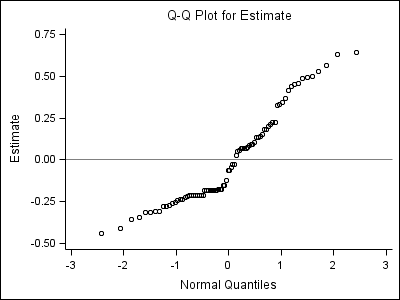
Table 7.6 on page 235. This is fairly long table comparing a lot of possible interaction terms with model presented in Table 7.3. We only present code for the first row of the table testing interaction term on age and lwt. The other rows of the table can be generated exactly the same way and we omit them here.
data table7_6;
   set lowbwt11a;
   agelwt = age*lwt;
run;
ods listing close;
proc mdc data = table7_6;
  model low = lwt smoke ptd ht ui /type = clogit nchoice=2;
  id pair;
  ods output  FitSummary = w_o_interacton;
run;
proc mdc data = table7_6;
  model low = lwt smoke ptd ht ui agelwt/type = clogit nchoice=2;
  id pair;
  ods output  FitSummary = w_interaction;
run;
ods listing;
proc sql;
  create table row1 as
  select w1.cvalue1 as w_o_ll, w2.cvalue1 as w_ll
  from w_o_interacton as w1, w_interaction as w2
  where w1.label1="Log Likelihood" & w2.label1="Log Likelihood";
quit;
data row1;
  set row1;
  g = 2*(w_ll - w_o_ll);
  p = 1-  PROBCHI(g, 1);
  output;
run;
proc print data = row1;
run;
Obs     w_o_ll        w_ll          t          p
 1     -26.23687    -25.98409    0.50556    0.47707
7.4 Assessment of fit in a matched study
As we have mentioned at the beginning of this chapter, SAS proc mdc does not offer diagnostic statistics. We follow the method discussed in the book using the difference variables.
Figure 7.2, Figure 7.3 and Figure 7.4.
data assess;
  set lowbwt11a;
  retain lwt1 smoke1 ptd1 ht1 ui1;
  by pair;
  if first.pair then do;
  lwt1 = lwt;
  smoke1 = smoke;
  ptd1 = ptd;
  ht1  = ht;
  ui1 = ui;
  end;
  else do;
  lwt1 = lwt - lwt1;
  smoke1 = smoke - smoke1;
  ptd1 = ptd - ptd1;
  ht1  = ht - ht1;
  ui1 = ui - ui1;
  output;
  end;
  keep low lwt1 smoke1 ptd1 ht1 ui1 ;
run;
proc logistic data = assess;
  model low = lwt1 smoke1 ptd1 ht1 ui1 /noint;
  output out = test difchisq = _dx2 c = dbeta  p = p ;
run;
goptions reset = all;
symbol v = circle c = black;
axis1 label = (a=90) minor = none;
proc gplot data = test;
  plot _dx2*p /vaxis = axis1;
  plot dbeta*p /vaxis=axis1;
  bubble _dx2*p = dbeta / bsize = 10 vaxis=axis1;
run;
quit;
Table 7.7 on page 240.
proc logistic data = assess;
  model low = lwt1 smoke1 ptd1 ht1 ui1 /noint;
  output out = test difchisq = _dx2 c = dbeta  p = p h = h ;
run;
proc print data = test (drop=_level_);
  where dbeta >.4;
  format lwt1 smoke1 ptd1 ht1 ui1 4.0 p dbeta difchisq _dx2 h 4.2;
run;
Obs    low    lwt1    smoke1    ptd1     ht1     ui1       p       h    dbeta    _dx2
  9     1       48       -1        0       0       0    0.10    0.05    0.50     9.53
 16     1      -49        1       -1       0      -1    0.31    0.24    0.92     2.92
 27     1       35        1        0      -1       0    0.20    0.20    1.25     4.97
 34     1       38       -1        0       0       0    0.11    0.05    0.42     8.19
Table 7.8 on page 241 .
proc logistic data = assess;
  model low = lwt1 smoke1 ptd1 ht1 ui1 /noint AGGREGATE scale=none;
run;
       Deviance and Pearson Goodness-of-Fit Statistics
Criterion        DF          Value     Value/DF     Pr > ChiSq
Deviance         51        52.4737       1.0289         0.4167
Pearson          51        50.7566       0.9952         0.4833
             Analysis of Maximum Likelihood Estimates
                               Standard          Wald
Parameter    DF    Estimate       Error    Chi-Square    Pr > ChiSq
lwt1          1     -0.0151     0.00815        3.4281        0.0641
smoke1        1      1.4796      0.5620        6.9305        0.0085
ptd1          1      1.6706      0.7468        5.0041        0.0253
ht1           1      2.3294      1.0025        5.3984        0.0202
ui1           1      1.3449      0.6938        3.7571        0.0526
data table7_8;
  set assess;
  id = _n_;
run;
proc logistic data = table7_8;
  model low = lwt1 smoke1 ptd1 ht1 ui1 /noint AGGREGATE scale=none;
  where id ~=9;
run;
       Deviance and Pearson Goodness-of-Fit Statistics
Criterion        DF          Value     Value/DF     Pr > ChiSq
Deviance         50        47.3316       0.9466         0.5811
Pearson          50        48.5205       0.9704         0.5329
             Analysis of Maximum Likelihood Estimates
                               Standard          Wald
Parameter    DF    Estimate       Error    Chi-Square    Pr > ChiSq
lwt1          1     -0.0196     0.00910        4.6473        0.0311
smoke1        1      1.8781      0.6545        8.2334        0.0041
ptd1          1      1.8831      0.8279        5.1732        0.0229
ht1           1      2.7193      1.1184        5.9123        0.0150
ui1           1      1.4979      0.7317        4.1904        0.0407

proc logistic data = table7_8;
  model low = lwt1 smoke1 ptd1 ht1 ui1 /noint AGGREGATE scale=none;
  where id ~=16;
run;

       Deviance and Pearson Goodness-of-Fit Statistics
Criterion        DF          Value     Value/DF     Pr > ChiSq
Deviance         50        49.4140       0.9883         0.4968
Pearson          50        46.3723       0.9274         0.6197
             Analysis of Maximum Likelihood Estimates
                               Standard          Wald
Parameter    DF    Estimate       Error    Chi-Square    Pr > ChiSq
lwt1          1     -0.0126     0.00836        2.2653        0.1323
smoke1        1      1.3907      0.5681        5.9933        0.0144
ptd1          1      2.1109      0.8577        6.0563        0.0139
ht1           1      2.4069      1.0304        5.4564        0.0195
ui1           1      1.7624      0.7886        4.9950        0.0254

proc logistic data = table7_8;
  model low = lwt1 smoke1 ptd1 ht1 ui1 /noint AGGREGATE scale=none;
  where id ~=27;
run;

       Deviance and Pearson Goodness-of-Fit Statistics
Criterion        DF          Value     Value/DF     Pr > ChiSq
Deviance         50        48.1354       0.9627         0.5485
Pearson          50        49.0020       0.9800         0.5134
             Analysis of Maximum Likelihood Estimates
                               Standard          Wald
Parameter    DF    Estimate       Error    Chi-Square    Pr > ChiSq
lwt1          1     -0.0211     0.00917        5.2675        0.0217
smoke1        1      1.3894      0.5888        5.5673        0.0183
ptd1          1      1.8071      0.7963        5.1497        0.0233
ht1           1      3.5595      1.4073        6.3977        0.0114
ui1           1      1.5107      0.7336        4.2412        0.0395

proc logistic data = table7_8;
  model low = lwt1 smoke1 ptd1 ht1 ui1 /noint AGGREGATE scale=none;
  where id ~=34;
run;
       Deviance and Pearson Goodness-of-Fit Statistics
Criterion        DF          Value     Value/DF     Pr > ChiSq
Deviance         50        47.6911       0.9538         0.5665
Pearson          50        50.3025       1.0060         0.4614

             Analysis of Maximum Likelihood Estimates
                               Standard          Wald
Parameter    DF    Estimate       Error    Chi-Square    Pr > ChiSq
lwt1          1     -0.0188     0.00896        4.3979        0.0360
smoke1        1      1.8548      0.6487        8.1742        0.0042
ptd1          1      1.8630      0.8191        5.1736        0.0229
ht1           1      2.6686      1.1029        5.8548        0.0155
ui1           1      1.4866      0.7284        4.1654        0.0413
Table 7.9 on page 242.
proc logistic data = table7_8;
  model low = lwt1 smoke1 ptd1 ht1 ui1 /noint clodds = wald;
  units lwt1 = 10;
run;

         Analysis of Maximum Likelihood Estimates
                               Standard          Wald
Parameter    DF    Estimate       Error    Chi-Square    Pr > ChiSq
lwt1          1     -0.0151     0.00815        3.4281        0.0641
smoke1        1      1.4796      0.5620        6.9305        0.0085
ptd1          1      1.6706      0.7468        5.0041        0.0253
ht1           1      2.3294      1.0025        5.3984        0.0202
ui1           1      1.3449      0.6938        3.7571        0.0526

           Odds Ratio Estimates
             Point          95% Wald
Effect    Estimate      Confidence Limits
lwt1         0.985       0.969       1.001
smoke1       4.391       1.459      13.212
ptd1         5.315       1.230      22.973
ht1         10.271       1.440      73.283
ui1          3.838       0.985      14.951
    Wald Confidence Interval for Adjusted Odds Ratios
Effect         Unit     Estimate     95% Confidence Limits
lwt1        10.0000        0.860        0.733        1.009
7.5 An example of the use of the logistic regression model in a 1-M matched study 
For this section, we omit the calculation of odds ratio after proc mdc. The calculation is shown in the first section of this chapter and is the same calculation here.
Table 7.11 on page 246.
proc mdc data = bbdm13;
  model fndx = chk /type = clogit nchoice=4;
  id str;
run;
Conditional Logit Estimates
             Model Fit Summary
Dependent Variable                     fndx
Number of Observations                   50
Number of Cases                         200
Log Likelihood                    -62.81737
Maximum Absolute Gradient        2.03546E-9
Number of Iterations                      4
Optimization Method          Newton-Raphson
AIC                               127.63473
Schwarz Criterion                 129.54676

           Goodness-of-Fit Measures for Discrete Choice Models
Measure                       Value    Formula
Likelihood Ratio (R)         12.995    2 * (LogL - LogL0)
Upper Bound of R (U)         138.63    - 2 * LogL0
Aldrich-Nelson               0.2063    R / (R+N)
Cragg-Uhler 1                0.2289    1 - exp(-R/N)
Cragg-Uhler 2                0.2441    (1-exp(-R/N)) / (1-exp(-U/N))
Estrella                     0.2388    1 - (1-R/U)^(U/N)
Adjusted Estrella            0.2048    1 - ((LogL-K)/LogL0)^(-2/N*LogL0)
McFadden's LRI               0.0937    R / U
Veall-Zimmermann             0.2807    (R * (U+N)) / (U * (R+N))
N = # of observations, K = # of regressors

                              Parameter Estimates
                                    Standard                 Approx
Parameter       DF     Estimate        Error    t Value    Pr > |t|    Gradient
chk              1      -1.2454       0.3815      -3.26      0.0011    -2.04E-9
proc mdc data = bbdm13;
  model fndx = agmn /type = clogit nchoice=4;
  id str;
run;
                              Parameter Estimates
                                    Standard                 Approx
Parameter       DF     Estimate        Error    t Value    Pr > |t|    Gradient
agmn             1       0.4718       0.1110       4.25      <.0001    1.21E-11
proc mdc data = bbdm13;
  model fndx = wt /type = clogit nchoice=4;
  id str;
run;
                              Parameter Estimates
                                    Standard                 Approx
Parameter       DF     Estimate        Error    t Value    Pr > |t|    Gradient
wt               1      -0.0352     0.008599      -4.09      <.0001    -5.76E-9
data bbdm13a;
  bbdm13;
  mst2 = ( mst = 2 | mst = 3);
  mst4 = ( mst = 4);
  mst5 = ( mst = 5);
run;
proc mdc data = bbdm13a;
  model fndx = mst2 mst4 mst5 /type = clogit nchoice=4;
  id str;
run;
                              Parameter Estimates
                                    Standard                 Approx
Parameter       DF     Estimate        Error    t Value    Pr > |t|    Gradient
mst2             1      -0.3584       0.5605      -0.64      0.5225    5.47E-11
mst4             1      -0.7510       0.7904      -0.95      0.3420    -364E-12
mst5             1       1.2484       0.6059       2.06      0.0393    9.22E-11
Table 7.12 on page 247.
proc mdc data = bbdm13;
  model fndx = chk agmn wt mst2 mst4 mst5 /type = clogit nchoice=4;
  id str;
run;
The MDC Procedure
Conditional Logit Estimates
             Model Fit Summary
Dependent Variable                     fndx
Number of Observations                   50
Number of Cases                         200
Log Likelihood                    -45.21482
Maximum Absolute Gradient        2.37731E-6
Number of Iterations                      5
Optimization Method          Newton-Raphson
AIC                               102.42965
Schwarz Criterion                 113.90179

                              Parameter Estimates
                                    Standard                 Approx
Parameter       DF     Estimate        Error    t Value    Pr > |t|    Gradient
chk              1      -1.1218       0.4474      -2.51      0.0122    -2.21E-8
agmn             1       0.3561       0.1292       2.76      0.0058    8.038E-8
wt               1      -0.0284     0.009978      -2.84      0.0045    -2.38E-6
mst2             1      -0.2030       0.6473      -0.31      0.7538    -3.36E-9
mst4             1      -0.4916       0.8173      -0.60      0.5475    -1.21E-9
mst5             1       1.4722       0.7582       1.94      0.0522    7.341E-9
Table 7.13 on page 247.
proc mdc data = bbdm13;
  model fndx = chk agmn wt mst5 /type = clogit nchoice=4;
  id str;
run;
The MDC Procedure
Conditional Logit Estimates
             Model Fit Summary
Dependent Variable                     fndx
Number of Observations                   50
Number of Cases                         200
Log Likelihood                    -45.43901
Maximum Absolute Gradient        2.22381E-6
Number of Iterations                      5
Optimization Method          Newton-Raphson
AIC                                98.87802
Schwarz Criterion                 106.52611

                              Parameter Estimates
                                    Standard                 Approx
Parameter       DF     Estimate        Error    t Value    Pr > |t|    Gradient
chk              1      -1.1613       0.4470      -2.60      0.0094       -2E-8
agmn             1       0.3592       0.1279       2.81      0.0050    7.529E-8
wt               1      -0.0282     0.009978      -2.83      0.0047    -2.22E-6
mst5             1       1.5934       0.7360       2.16      0.0304    6.713E-9
7.7 An example of assessment of fit in a 1-M matched study
Currently, SAS does not offer the diagnostics discussed in this section. Stata has an add-on program called clfit that will generate these diagnostic variables after clogit. Please see Chapter 7 in Stata for more detail.