8.1 The multinomial logistic regression model
This section uses the data set https://stats.idre.ucla.edu/wp-content/uploads/2016/02/meexp.sas7bdat on mammography experience study. You can download it following the link. Table 8.2 on page 266.
proc freq data = meexp;
  where me ~=2;
  tables me*hist /norow nocol nopercent relrisk;
run;
proc freq data = meexp;
  where me ~=1;
  tables me*hist /norow nocol nopercent relrisk;
run;

The FREQ Procedure
Table of me by hist
me        hist
Frequency|       0|       1|  Total
---------+--------+--------+
       0 |    220 |     14 |    234
---------+--------+--------+
       1 |     85 |     19 |    104
---------+--------+--------+
Total         305       33      338

Statistics for Table of me by hist
           Estimates of the Relative Risk (Row1/Row2)
Type of Study                   Value       95% Confidence Limits
-----------------------------------------------------------------
Case-Control (Odds Ratio)      3.5126        1.6855        7.3205
Cohort (Col1 Risk)             1.1503        1.0446        1.2668
Cohort (Col2 Risk)             0.3275        0.1709        0.6277
Sample Size = 338

The FREQ Procedure
Table of me by hist
me        hist
Frequency|       0|       1|  Total
---------+--------+--------+
       0 |    220 |     14 |    234
---------+--------+--------+
       2 |     63 |     11 |     74
---------+--------+--------+
Total         283       25      308

Statistics for Table of me by hist
           Estimates of the Relative Risk (Row1/Row2)
Type of Study                   Value       95% Confidence Limits
-----------------------------------------------------------------
Case-Control (Odds Ratio)      2.7438        1.1870        6.3421
Cohort (Col1 Risk)             1.1043        0.9987        1.2211
Cohort (Col2 Risk)             0.4025        0.1910        0.8480
Sample Size = 308
Table 8.3 on page 267.
proc logistic data = meexp;
  class me (ref="0");
  model me = hist /link=glogit;
run;

The LOGISTIC Procedure
        Testing Global Null Hypothesis: BETA=0
Test                 Chi-Square       DF     Pr > ChiSq
Likelihood Ratio        12.8581        2         0.0016
Score                   13.0502        2         0.0015
Wald                    12.0106        2         0.0025

       Type III Analysis of Effects
                        Wald
Effect      DF    Chi-Square    Pr > ChiSq
hist         2       12.0106        0.0025

                Analysis of Maximum Likelihood Estimates
                                     Standard          Wald
Parameter    me    DF    Estimate       Error    Chi-Square    Pr > ChiSq
Intercept    1      1     -0.9510      0.1277       55.4474        <.0001
Intercept    2      1     -1.2505      0.1429       76.5842        <.0001
hist         1      1      1.2564      0.3747       11.2448        0.0008
hist         2      1      1.0093      0.4275        5.5744        0.0182

                 Odds Ratio Estimates
                         Point          95% Wald
Effect    me          Estimate      Confidence Limits
hist      1              3.513       1.685       7.320
hist      2              2.744       1.187       6.342
Table 8.4 on page 269 for estimated covariance matrix from the fitted model in Table 8.3. We only display the output for covariance matrix, the other part of the output will be the same as in previous table and will be omitted. The only difference in the code is the use of the option covb in the model statement.
proc logistic data = meexp;
  class me (ref="0");
  model me = hist /link=glogit covb;
run;
                      Estimated Covariance Matrix
                 Intercept_      Intercept_
Variable                  1               2        hist_1        hist_2
Intercept_1         0.01631        0.004545      -0.01631      -0.00455
Intercept_2        0.004545        0.020418      -0.00455      -0.02042
hist_1             -0.01631        -0.00455       0.14037      0.075974
hist_2             -0.00455        -0.02042      0.075974      0.182756
Table 8.5 on page 271, cross-classification of mammography experience (me) by detc.
proc freq data = meexp;
  table me*detc /norow nocol nopercent;
run;
Table of me by detc
me        detc
Frequency|       1|       2|       3|  Total
---------+--------+--------+--------+
       0 |     13 |     77 |    144 |    234
---------+--------+--------+--------+
       1 |      1 |     12 |     91 |    104
---------+--------+--------+--------+
       2 |      4 |     16 |     54 |     74
---------+--------+--------+--------+
Total          18      105      289      412
Table 8.6 page 271, results of fitting the logistic regression model to the data in Table 8.5.
proc logistic data = meexp ;
  class me(ref="0") detc (ref="1") / coding = reference;
  model me = detc /link = glogit;
run;

             Analysis of Maximum Likelihood Estimates
                                       Standard          Wald
Parameter      me    DF    Estimate       Error    Chi-Square    Pr > ChiSq
Intercept      1      1     -2.5649      1.0377        6.1091        0.0134
Intercept      2      1     -1.1787      0.5718        4.2494        0.0393
detc      2    1      1      0.7060      1.0831        0.4248        0.5145
detc      2    2      1     -0.3926      0.6344        0.3830        0.5360
detc      3    1      1      2.1059      1.0463        4.0509        0.0441
detc      3    2      1      0.1978      0.5936        0.1111        0.7389

                   Odds Ratio Estimates
                              Point          95% Wald
Effect         me          Estimate      Confidence Limits
detc 2 vs 1    1              2.026       0.242      16.927
detc 2 vs 1    2              0.675       0.195       2.341
detc 3 vs 1    1              8.215       1.057      63.860
detc 3 vs 1    2              1.219       0.381       3.901
Table 8.7 on page 274 and tests for equality of the coefficients of sympt for category 3 and 4 within each logit. When a variable is declared to be a categorical variable, SAS proc logistic creates corresponding dummy variables and names them in a systematical way. For example, there are six dummy variables created for variable sympt and they are sympt2_1, sympt2_2, sympt3_1, sympt3_2, sympt4_1 and sympt4_2, because there are two equations to be estimated and sympt has four categories, with reference category being 1.
proc logistic data = meexp ;
  class  me(ref="0") sympt(ref="1") detc(ref="1") /coding=reference;
  model me = sympt pb hist bse detc /link = glogit;
run;
                 Analysis of Maximum Likelihood Estimates
                                       Standard          Wald
Parameter      me    DF    Estimate       Error    Chi-Square    Pr > ChiSq
Intercept      1      1     -2.9973      1.5389        3.7937        0.0514
Intercept      2      1     -0.9861      1.1118        0.7865        0.3751
sympt     2    1      1      0.1098      0.9226        0.0142        0.9052
sympt     2    2      1     -0.2901      0.6441        0.2029        0.6524
sympt     3    1      1      1.9242      0.7774        6.1258        0.0133
sympt     3    2      1      0.8173      0.5398        2.2925        0.1300
sympt     4    1      1      2.4565      0.7752       10.0422        0.0015
sympt     4    2      1      1.1322      0.5477        4.2739        0.0387
pb             1      1     -0.2194      0.0755        8.4444        0.0037
pb             2      1     -0.1482      0.0764        3.7662        0.0523
hist           1      1      1.3662      0.4375        9.7512        0.0018
hist           2      1      1.0654      0.4594        5.3786        0.0204
bse            1      1      1.2916      0.5299        5.9416        0.0148
bse            2      1      1.0521      0.5150        4.1739        0.0411
detc      2    1      1      0.0161      1.1615        0.0002        0.9889
detc      2    2      1     -0.9244      0.7138        1.6774        0.1953
detc      3    1      1      0.9032      1.1264        0.6429        0.4226
detc      3    2      1     -0.6906      0.6871        1.0100        0.3149

proc logistic data = meexp ;
  class  me(ref="0") sympt(ref="1") detc(ref="1") /coding=reference;
  model me = sympt pb hist bse detc /link = glogit aggregate;
  test sympt3_1 = sympt4_1;
  test sympt3_2 = sympt4_2;
run;

      Linear Hypotheses Testing Results
                   Wald
 Label       Chi-Square      DF    Pr > ChiSq
 Test 1          3.2840       1        0.0700
 Test 2          0.9304       1        0.3348
Table 8.8 on page 275.
data table8_8;
  set meexp;
if sympt = 1 or sympt = 2 then symptd = 0 ;
else symptd = 1;
run;
proc logistic data = table8_8 ;
  class  me(ref="0")  detc(ref="1") /coding=reference;
  model me = symptd pb hist bse detc /link = glogit;
run;

The LOGISTIC Procedure
       Type III Analysis of Effects
                        Wald
Effect      DF    Chi-Square    Pr > ChiSq
symptd       2       27.0465        <.0001
pb           2       13.5308        0.0012
hist         2        9.4435        0.0089
bse          2        8.1510        0.0170
detc         4        8.0257        0.0906

                 Analysis of Maximum Likelihood Estimates
                                       Standard          Wald
Parameter      me    DF    Estimate       Error    Chi-Square    Pr > ChiSq
Intercept      1      1     -2.7024      1.4341        3.5510        0.0595
Intercept      2      1     -0.9987      1.0720        0.8680        0.3515
symptd         1      1      2.0950      0.4573       20.9842        <.0001
symptd         2      1      1.1214      0.3572        9.8552        0.0017
pb             1      1     -0.2510      0.0729       11.8454        0.0006
pb             2      1     -0.1681      0.0742        5.1366        0.0234
hist           1      1      1.2933      0.4335        8.8990        0.0029
hist           2      1      1.0140      0.4538        4.9932        0.0254
bse            1      1      1.2439      0.5263        5.5863        0.0181
bse            2      1      1.0286      0.5140        4.0049        0.0454
detc      2    1      1      0.0893      1.1606        0.0059        0.9386
detc      2    2      1     -0.9022      0.7146        1.5936        0.2068
detc      3    1      1      0.9719      1.1259        0.7451        0.3880
detc      3    2      1     -0.6698      0.6876        0.9490        0.3300
Table 8.9 on page 276, estimated coefficients, estimated standard errors, Wald statistics and two-tailed p-values for the model fit excluding detc to the mammography experience data.
proc logistic data = table8_8 ;
  class  me(ref="0")   /coding=reference;
  model me = symptd  pb hist bse  /link = glogit;
run;
                Analysis of Maximum Likelihood Estimates
                                     Standard          Wald
Parameter    me    DF    Estimate       Error    Chi-Square    Pr > ChiSq
Intercept    1      1     -1.7885      0.8470        4.4584        0.0347
Intercept    2      1     -1.7421      0.8087        4.6410        0.0312
symptd       1      1      2.2302      0.4519       24.3538        <.0001
symptd       2      1      1.1531      0.3514       10.7697        0.0010
pb           1      1     -0.2825      0.0713       15.6819        <.0001
pb           2      1     -0.1578      0.0712        4.9144        0.0266
hist         1      1      1.2966      0.4293        9.1223        0.0025
hist         2      1      1.0613      0.4527        5.4969        0.0191
bse          1      1      1.2209      0.5210        5.4910        0.0191
bse          2      1      0.9604      0.5072        3.5853        0.0583
Table 8.10 on page 277, estimated coefficients, estimated standard errors, Wald statistics and two-tailed p-values for the model fit using detcd to the mammography experience data.
data table8_10;
  set table8_8;
    detcd = (detc =3);
run;
proc logistic data = table8_10 ;
  class  me(ref="0")  /coding=reference;
  model me = symptd  pb hist bse  detcd/ link = glogit ;
run;

       Type III Analysis of Effects
                        Wald
Effect      DF    Chi-Square    Pr > ChiSq
symptd       2       27.1306        <.0001
pb           2       13.1529        0.0014
hist         2        9.8217        0.0074
bse          2        7.7204        0.0211
detcd        2        6.2864        0.0431

                Analysis of Maximum Likelihood Estimates
                                     Standard          Wald
Parameter    me    DF    Estimate       Error    Chi-Square    Pr > ChiSq
Intercept    1      1     -2.6233      0.9263        8.0196        0.0046
Intercept    2      1     -1.8239      0.8551        4.5495        0.0329
symptd       1      1      2.0944      0.4574       20.9692        <.0001
symptd       2      1      1.1274      0.3564       10.0086        0.0016
pb           1      1     -0.2495      0.0726       11.8151        0.0006
pb           2      1     -0.1543      0.0726        4.5155        0.0336
hist         1      1      1.3098      0.4336        9.1258        0.0025
hist         2      1      1.0632      0.4528        5.5121        0.0189
bse          1      1      1.2369      0.5254        5.5425        0.0186
bse          2      1      0.9560      0.5073        3.5508        0.0595
detcd        1      1      0.8851      0.3562        6.1741        0.0130
Figure 8.1 on page 278, plot of the estimated logistic regression coefficients for the quartile design variables created from pb for Logit 1 (o) and Logit 2 (delta).
data figure8_1;
  set table8_10;
  pb1 = (pb = 5);
  pb2 = (6<= pb <= 7);
  pb3 = (8 <=pb <=9);
  pb4 = (pb >=10);
run;
proc logistic data = figure8_1 ;
  class  me(ref="0")  / coding=reference;
  model me = pb2 - pb4 symptd hist bse detcd / link = glogit ;
  ods output Parameterestimates = fig8_1;
run;
data fig8_1a;
  set fig8_1;
  if variable = "Intercept" then do; variable = "pb1"; x = 5; estimate = 0; end;
  if variable = "pb2" then x = 6.5;
  if variable = "pb3" then x = 8.5;
  if variable = "pb4" then x = 13.5;
  if variable in ("pb1", "pb2", "pb3", "pb4");
  keep x estimate response;
run;
symbol i = join r = 2 value=circle;
axis1 order = (-1.5 to 0 by .5) minor = none label = (a=90 'Estimated Logit');
axis2 minor = none label = ('Perceived Benefit');
proc gplot data = fig8_1a;
  format estimate 4.2;
  plot estimate*x = response /vaxis = axis1 haxis=axis2;
run;
quit;
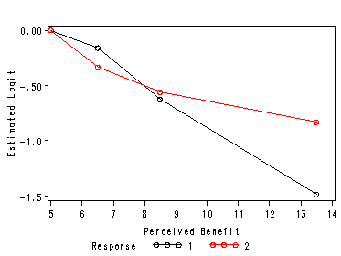
Table 8.11 on page 280, comparison of the maximum likelihood estimates, MLE, and the estimates from individual logistic regression fits, ILR.
NOTE: This gives the values for the columns labeled MLE.
proc logistic data = table8_10 ;
  class  me(ref="0")  /coding=reference;
  model me = symptd  pb hist bse  detcd/ link = glogit ;
run;
                Analysis of Maximum Likelihood Estimates
                                     Standard          Wald
Parameter    me    DF    Estimate       Error    Chi-Square    Pr > ChiSq
Intercept    1      1     -2.6233      0.9263        8.0196        0.0046
Intercept    2      1     -1.8239      0.8551        4.5495        0.0329
symptd       1      1      2.0944      0.4574       20.9692        <.0001
symptd       2      1      1.1274      0.3564       10.0086        0.0016
pb           1      1     -0.2495      0.0726       11.8151        0.0006
pb           2      1     -0.1543      0.0726        4.5155        0.0336
hist         1      1      1.3098      0.4336        9.1258        0.0025
hist         2      1      1.0632      0.4528        5.5121        0.0189
bse          1      1      1.2369      0.5254        5.5425        0.0186
bse          2      1      0.9560      0.5073        3.5508        0.0595
detcd        1      1      0.8851      0.3562        6.1741        0.0130
NOTE: This gives the values for the columns labeled ILR.
proc logistic data = table8_10 ;
 where me ~=2;
 model me(event="1") = symptd  pb hist bse  detcd/ link = glogit ;
run;
               Analysis of Maximum Likelihood Estimates
                                     Standard          Wald
Parameter    me    DF    Estimate       Error    Chi-Square    Pr > ChiSq
Intercept    1      1     -2.7651      0.9422        8.6129        0.0033
symptd       1      1      2.0910      0.4651       20.2098        <.0001
pb           1      1     -0.2426      0.0738       10.8203        0.0010
hist         1      1      1.3850      0.4683        8.7487        0.0031
bse          1      1      1.3633      0.5339        6.5203        0.0107
detcd        1      1      0.8527      0.3655        5.4440        0.0196

proc logistic data = table8_10 ;
  where me ~= 1;
  model me(event="2") = symptd  pb hist bse  detcd/ link = glogit ;
run;

                Analysis of Maximum Likelihood Estimates
                                     Standard          Wald
Parameter    me    DF    Estimate       Error    Chi-Square    Pr > ChiSq
Intercept    2      1     -1.8381      0.8600        4.5677        0.0326
symptd       2      1      1.1530      0.3566       10.4554        0.0012
pb           2      1     -0.1538      0.0726        4.4859        0.0342
hist         2      1      1.0977      0.4593        5.7107        0.0169
bse          2      1      0.9535      0.5097        3.4990        0.0614
detcd        2      1      0.0987      0.3191        0.0957        0.7571
Table 8.12 page 281, summary goodness-of-fit statistics (p-value) for the individual logistic regressions. SAS does not compute Stukel statistic and it has to be computed by hand. We also notice that for the Hosmer and Lemeshow goodness-of-fit test, SAS gives different results from Stata. In order to get the Pearson chi-square test statistic, we need to use option "aggregate scale = none" on the model statement.
proc logistic data = table8_10 ;
 where me ~=2;
 model me(event="1") = symptd  pb hist bse  detcd / aggregate scale=none link = glogit lackfit ;
run;

       Deviance and Pearson Goodness-of-Fit Statistics
Criterion        DF          Value     Value/DF     Pr > ChiSq
Deviance         68        44.7264       0.6577         0.9869
Pearson          68        67.8364       0.9976         0.4828
Hosmer and Lemeshow Goodness-of-Fit Test
Chi-Square       DF     Pr > ChiSq
    9.0594        8         0.3373

proc logistic data = table8_10 ;
  where me ~= 1;
  model me(event="2") = symptd  pb hist bse  detcd / aggregate scale=none link = glogit lackfit;
run;

 Deviance and Pearson Goodness-of-Fit Statistics
Criterion        DF          Value     Value/DF     Pr > ChiSq
Deviance         69        64.3934       0.9332         0.6346
Pearson          69        63.8266       0.9250         0.6535
Number of unique profiles: 75
Hosmer and Lemeshow Goodness-of-Fit Test
Chi-Square       DF     Pr > ChiSq
   13.6511        8         0.0913
Table 8.13 on page 283. Notice that the examples in the book were originally done in Stata. In Stata, the diagnostic statistics are computed based on the covariate patterns, not on the individual observations. In SAS, we can do the same by collapsing the data up to covariate pattern level. Also notice that the difference in deviance residual is calculated differently and we will compute it the Stata way in a data step.
proc sql;
  create table event_trial as
  select distinct symptd, pb, hist, bse, detcd, sum(me) as events, count(me) as trials
  from table8_10
  where me ^=2
  group by symptd, pb, hist, bse, detcd;
quit;
proc logistic data = event_trial ;
 model events/trials = symptd  pb hist bse  detcd /  ;
 output out = table8_13 p = p resdev = d c=db difchisq = dx2 difdev = dd  h = h;
run;

data table8_13a;
  set table8_13;
  newdd = d**2/(1-h);
run;
proc print data = table8_13a noobs;
where dx2 >7;
var symptd pb hist bse detcd events trials p db dx2 newdd  h ;
run;

symptd pb hist bse detcd events trials    p       db     dx2    newdd     h
   0    6   0   0    0      1      2   0.01447 0.54330 33.5851 5.81993 0.01592
   1    9   0   1    1     11     18   0.34488 1.73273  7.0371 6.58556 0.19758

proc sort data = table8_10;
  by symptd ph hist bse detcd;
run; /*to create pattern number in the order of predictors*/
proc sql;
  create table event_trial as
  select distinct symptd, pb, hist, bse, detcd, sum(me=2) as events, count(me) as trials
  from table8_10
  where me ^=1
  group by symptd, pb, hist, bse, detcd;
quit;
data event_trial;
  set event_trial;
  pattern = _n_;
run;
proc logistic data = event_trial ;
 model events/trials = symptd  pb hist bse  detcd /  ;
 output out = table8_13 p = p resdev = d c=db difchisq = dx2 difdev = dd  h = h;
run;
proc print data = table8_13a;
run;
data table8_13a;
  set table8_13;
  newdd = d**2/(1-h);
run;
proc print data = table8_13a noobs;
where pattern = 62 | pattern = 63 | pattern = 66;
var symptd pb hist bse detcd events trials p db dx2 newdd  h ;
run;

symptd pb hist bse detcd events trials    p       db     dx2    newdd     h
   1    9   1   1    0      3      3   0.49554 0.95641 3.81886 5.26768 0.20028
   1   10   0   0    0      1      1   0.09772 0.26399 9.49004 4.78066 0.02706
   1   10   0   1    1      2     19   0.23675 0.99901 2.53433 3.01400 0.28274
page 285 Table 8.14 Estimated coefficients, estimated standard errors, Wald statistics and two-tailed p-values for the model fit after deleting 40 subjects corresponding to covariate patterns 62, 63, and 66 in Table 8.13. In the previous example, we collapsed data into covariate patterns and used the event/trial syntax in proc logistic. Now we have to identify the covariate patterns first and use the option link = glogit to perform the multinomial logistic regression. The two calls to proc sql below created covariate patterns for each pairs of the output. We then merge them back with the original data set.
proc sort data = table8_10;
  by symptd pb hist bse detcd;
run;
proc sql;
  create table event_trial1 as
  select distinct symptd, pb, hist, bse, detcd
  from table8_10
  where me ^=2
  group by symptd, pb, hist, bse, detcd;
quit;
proc sql;
  create table event_trial2 as
  select distinct symptd, pb, hist, bse, detcd
  from table8_10
  where me ^=1
  group by symptd, pb, hist, bse, detcd;
quit;
data event_trial1;
  set event_trial1;
  pattern1 = _n_;
run;
data event_trial2;
  set event_trial2;
  pattern2 = _n_;
run;
data table8_14;
  merge  table8_10 event_trial1 event_trial2 ;
  by  symptd pb hist bse detcd;
run;
proc logistic data = table8_14;
  where ~(pattern1 =63 & (me = 0 | me = 1) ) & ~( pattern2 = 62 & (me = 0 | me =2)) &
         ~(pattern2 = 66 & (me = 0 | me =2));
  class me(ref="0");
  model me = symptd pb hist bse detcd /link=glogit;
run;
                Analysis of Maximum Likelihood Estimates
                                     Standard          Wald
Parameter    me    DF    Estimate       Error    Chi-Square    Pr > ChiSq
Intercept    1      1     -2.8916      1.0416        7.7069        0.0055
Intercept    2      1     -2.6637      0.9557        7.7688        0.0053
symptd       1      1      2.1244      0.4633       21.0280        <.0001
symptd       2      1      1.1906      0.3610       10.8779        0.0010
pb           1      1     -0.2163      0.0854        6.4097        0.0114
pb           2      1     -0.0804      0.0786        1.0455        0.3065
hist         1      1      1.2435      0.4418        7.9232        0.0049
hist         2      1      0.6059      0.4952        1.4969        0.2212
bse          1      1      1.2712      0.5310        5.7311        0.0167
bse          2      1      1.0812      0.5123        4.4543        0.0348
detcd        1      1      0.8830      0.3691        5.7221        0.0168
detcd        2      1      0.4768      0.3404        1.9620        0.1613
Page 286 Table 8.15 Estimated odds ratios and 95% confidence intervals for factors associated with use of mammography screening.
proc logistic data = table8_14;
  class me(ref="0");
  model me = symptd pb hist bse detcd /link=glogit CLODDS=wald;
  units pb =-2;
run;

                 Odds Ratio Estimates
                         Point          95% Wald
Effect    me          Estimate      Confidence Limits
symptd    1              8.121       3.313      19.902
symptd    2              3.088       1.536       6.208
pb        1              0.779       0.676       0.898
pb        2              0.857       0.743       0.988
hist      1              3.706       1.584       8.668
hist      2              2.896       1.192       7.034
bse       1              3.445       1.230       9.648
bse       2              2.601       0.962       7.031
detcd     1              2.423       1.206       4.871
detcd     2              1.121       0.601       2.091

           Wald Confidence Interval for Adjusted Odds Ratios
Effect     me               Unit     Estimate     95% Confidence Limits
pb         1             -2.0000        1.647        1.239        2.189
pb         2             -2.0000        1.362        1.024        1.810
8.2 Ordinal logistic regression models
page 293 Table 8.16 Cross-classification of the four category ordinal scale birth weight outcome versus smoking status of the mother.
data bwt;
  set lowbwt;
  if bwt >3500 then bcat = 0;
  else if 3000 < bwt <= 3500 then bcat = 1;
  else if 2500 < bwt <= 3000 then bcat = 2;
  else  bcat = 3;
run;
proc freq data= bwt;
  tables bcat*smoke / nopercent nocol norow;
run;

bcat      smoke
Frequency|       0|       1|  Total
---------+--------+--------+
       0 |     35 |     11 |     46
---------+--------+--------+
       1 |     29 |     17 |     46
---------+--------+--------+
       2 |     22 |     16 |     38
---------+--------+--------+
       3 |     29 |     30 |     59
---------+--------+--------+
Total         115       74      189
Middle of page
proc freq data= bwt;
  where bcat = 0 | bcat = 1;
  tables bcat*smoke /norow nocol nopercent relrisk;
run;
Table of bcat by smoke
bcat      smoke
Frequency|       0|       1|  Total
---------+--------+--------+
       0 |     35 |     11 |     46
---------+--------+--------+
       1 |     29 |     17 |     46
---------+--------+--------+
Total          64       28       92

Statistics for Table of bcat by smoke
           Estimates of the Relative Risk (Row1/Row2)
Type of Study                   Value       95% Confidence Limits
-----------------------------------------------------------------
Case-Control (Odds Ratio)      1.8652        0.7552        4.6065
Cohort (Col1 Risk)             1.2069        0.9174        1.5877
Cohort (Col2 Risk)             0.6471        0.3416        1.2258
Sample Size = 92
proc freq data= bwt;
  where bcat = 0 | bcat = 2;
  tables bcat*smoke /norow nocol nopercent relrisk;
run;

Table of bcat by smoke
bcat      smoke
Frequency|       0|       1|  Total
---------+--------+--------+
       0 |     35 |     11 |     46
---------+--------+--------+
       2 |     22 |     16 |     38
---------+--------+--------+
Total          57       27       84

Statistics for Table of bcat by smoke
           Estimates of the Relative Risk (Row1/Row2)
Type of Study                   Value       95% Confidence Limits
-----------------------------------------------------------------
Case-Control (Odds Ratio)      2.3140        0.9087        5.8927
Cohort (Col1 Risk)             1.3142        0.9583        1.8024
Cohort (Col2 Risk)             0.5679        0.3006        1.0730
Sample Size = 84
proc freq data= bwt;
  where bcat = 0 | bcat = 3;
  tables bcat*smoke /norow nocol nopercent relrisk;
run;

Table of bcat by smoke
bcat      smoke
Frequency|       0|       1|  Total
---------+--------+--------+
       0 |     35 |     11 |     46
---------+--------+--------+
       3 |     29 |     30 |     59
---------+--------+--------+
Total          64       41      105

Statistics for Table of bcat by smoke
           Estimates of the Relative Risk (Row1/Row2)
Type of Study                   Value       95% Confidence Limits
-----------------------------------------------------------------
Case-Control (Odds Ratio)      3.2915        1.4093        7.6874
Cohort (Col1 Risk)             1.5480        1.1400        2.1020
Cohort (Col2 Risk)             0.4703        0.2651        0.8343
Sample Size = 105
proc logistic data = bwt;
  class bcat (ref="0");
  model bcat(event="0") = smoke /link = glogit;
run;

                 Analysis of Maximum Likelihood Estimates
                                       Standard          Wald
Parameter    bcat    DF    Estimate       Error    Chi-Square    Pr > ChiSq
Intercept    1        1     -0.1881      0.2511        0.5608        0.4539
Intercept    2        1     -0.4643      0.2721        2.9122        0.0879
Intercept    3        1     -0.1881      0.2511        0.5608        0.4539
smoke        1        1      0.6234      0.4613        1.8262        0.1766
smoke        2        1      0.8390      0.4769        3.0950        0.0785
smoke        3        1      1.1914      0.4328        7.5779        0.0059

                 Odds Ratio Estimates
                         Point          95% Wald
Effect    bcat        Estimate      Confidence Limits
smoke     1              1.865       0.755       4.607
smoke     2              2.314       0.909       5.893
smoke     3              3.292       1.409       7.687
Result of adjacent-category logits on page 294 and page 295.
proc catmod data = bwt;
  population smoke;
  response alogits;
  model bcat = (0 1 0 0,
                0 0 1 0,
                0 0 0 1,
                1 1 0 0,
                1 0 1 0,
                1 0 0 1) ;
run;
quit;

The CATMOD Procedure
                Response Functions and Design Matrix
          Function      Response              Design Matrix
Sample     Number       Function        1        2        3        4
--------------------------------------------------------------------
    1          1        -0.18805        0        1        0        0
               2        -0.27625        0        0        1        0
               3         0.27625        0        0        0        1
    2          1         0.43532        1        1        0        0
               2        -0.06062        1        0        1        0
               3         0.62861        1        0        0        1

            Analysis of Variance
Source         DF   Chi-Square    Pr > ChiSq
--------------------------------------------
Model|Mean      3        11.75        0.0083
Residual        2         0.33        0.8460

            Analysis of Weighted Least Squares Estimates
                                  Standard        Chi-
Effect    Parameter    Estimate      Error      Square    Pr > ChiSq
--------------------------------------------------------------------
Model          1         0.3684     0.1346        7.49        0.0062
               2        -0.1088     0.2104        0.27        0.6051
               3        -0.3333     0.2254        2.19        0.1391
               4         0.2670     0.2205        1.47        0.2259
Page 296, Table 8.18 Unconstrained continuation-ratio model.
NOTE: Logit 1:
proc logistic data = bwt;
   where bcat = 0 | bcat = 1;
   model bcat (event="1") = smoke;
run;
             Analysis of Maximum Likelihood Estimates
                               Standard          Wald
Parameter    DF    Estimate       Error    Chi-Square    Pr > ChiSq
Intercept     1     -0.1881      0.2511        0.5608        0.4539
smoke         1      0.6234      0.4613        1.8262        0.1766
NOTE: Logit 2:
data bwt2;
  set bwt;
  if (bcat = 0 | bcat = 1) then bcat2 = 0;
  else if bcat = 2 then bcat2 = 1;
run;
proc logistic data = bwt2;
   model bcat2 (event="1") = smoke;
run;

             Analysis of Maximum Likelihood Estimates
                               Standard          Wald
Parameter    DF    Estimate       Error    Chi-Square    Pr > ChiSq
Intercept     1     -1.0678      0.2471       18.6685        <.0001
smoke         1      0.5083      0.3991        1.6218        0.2028
NOTE: Logit 3:
data bwt3;
  set bwt;
  if (bcat = 3) then bcat3 = 1;
  else bcat3 = 0;
run;
proc logistic data = bwt3;
   model bcat3 (event="1") = smoke;
run;

             Analysis of Maximum Likelihood Estimates
                               Standard          Wald
Parameter    DF    Estimate       Error    Chi-Square    Pr > ChiSq
Intercept     1     -1.0870      0.2147       25.6244        <.0001
smoke         1      0.7040      0.3196        4.8516        0.0276
Table 8.19 on page 297, estimated coefficients, standard errors, z-scores, two-tailed p-values for the fitted constrained continuation-ratio model. We will follow strategy described in chapter 6 of Logistic Regression Using the SAS System by Allison.
data first;
  set bwt;
  stage1 = 1;
  stage2 = 0;
  stage3 = 0;
  adv = bcat < 3;
run;
data second;
  set bwt;
  stage1 = 0;
  stage2 = 1;
  stage3 = 0;
  if bcat = 3 then delete;
  adv = bcat < 2;
run;
data third;
  set bwt;
  stage1 = 0;
  stage2 = 0;
  stage3 = 1;
  if bcat >=2 then delete;
  adv = bcat < 1;
run;
data concat;
  set first second third;
run;
proc logistic data = concat  ;
 model adv = stage1-stage3 smoke /noint ;
run;

             Analysis of Maximum Likelihood Estimates
                               Standard          Wald
Parameter    DF    Estimate       Error    Chi-Square    Pr > ChiSq
stage1        1     -1.0523      0.1862       31.9342        <.0001
stage2        1     -1.1138      0.2130       27.3565        <.0001
stage3        1     -0.1890      0.2204        0.7351        0.3912
smoke         1      0.6266      0.2192        8.1692        0.0043
page 303 Table 8.20 Results of fitting the proportional odds model to the four category birth weight outcome, BWT4N, with covariate LWT. Notice that SAS uses a model that does not negate the coefficient in equation (8.16) on page 291. This is why we have the coefficient for lwt being negative in the result.
proc logistic data = bwt descending;
  model bcat = lwt ;
run;

        Testing Global Null Hypothesis: BETA=0
Test                 Chi-Square       DF     Pr > ChiSq
Likelihood Ratio         9.0090        1         0.0027
Score                    9.2318        1         0.0024
Wald                     8.2081        1         0.0042

              Analysis of Maximum Likelihood Estimates
                                 Standard          Wald
Parameter      DF    Estimate       Error    Chi-Square    Pr > ChiSq
Intercept 3     1      0.8320      0.5857        2.0181        0.1554
Intercept 2     1      1.7073      0.5937        8.2707        0.0040
Intercept 1     1      2.8315      0.6176       21.0210        <.0001
lwt             1     -0.0127     0.00445        8.2081        0.0042
page 304 Table 8.21 Results of fitting the proportional odds model to the four category birth weight outcome, BWT4N, with covariate SMOKE.
proc logistic data = bwt descending;
  model bcat = smoke ;
run;

        Testing Global Null Hypothesis: BETA=0
Test                 Chi-Square       DF     Pr > ChiSq
Likelihood Ratio         7.9594        1         0.0048
Score                    7.9042        1         0.0049
Wald                     7.7800        1         0.0053

              Analysis of Maximum Likelihood Estimates
                                 Standard          Wald
Parameter      DF    Estimate       Error    Chi-Square    Pr > ChiSq
Intercept 3     1     -1.1163      0.1981       31.7641        <.0001
Intercept 2     1     -0.2477      0.1808        1.8764        0.1707
Intercept 1     1      0.8667      0.1928       20.2055        <.0001
smoke           1      0.7608      0.2728        7.7800        0.0053
8.2.2 Model building strategies for ordinal logistic regression models
page 306 Table 8.22 Results of fitting the proportional odds model to the four category birth weight outcome, BWT4N.
data bwt1;
  set bwt;
  ptd1 = (ptd >0);
run;
proc logistic data = bwt1 descending;
  class race(ref="1") /coding=reference;
  model bcat = age lwt race smoke ht ui ptd1 ;
run;

              Analysis of Maximum Likelihood Estimates
                                 Standard          Wald
Parameter      DF    Estimate       Error    Chi-Square    Pr > ChiSq
Intercept 3     1     -0.4956      0.9004        0.3030        0.5820
Intercept 2     1      0.5158      0.8995        0.3288        0.5664
Intercept 1     1      1.8031      0.9099        3.9273        0.0475
age             1    -0.00063      0.0274        0.0005        0.9818
lwt             1     -0.0129     0.00501        6.6337        0.0100
race      2     1      1.4708      0.4476       10.7985        0.0010
race      3     1      0.8693      0.3344        6.7597        0.0093
smoke           1      0.9877      0.3135        9.9244        0.0016
ht              1      1.1937      0.5916        4.0708        0.0436
ui              1      0.9130      0.4077        5.0134        0.0252
ptd1            1      0.8221      0.4075        4.0687        0.0437
proc logistic data = bwt1 descending;
  class race(ref="1") /coding=reference;
  model bcat = age lwt race smoke ht ui ptd1 /clodds = wald ;
  units age = 10 lwt = 10;
run;

              Odds Ratio Estimates
                   Point          95% Wald
Effect          Estimate      Confidence Limits
age                0.999       0.947       1.055
lwt                0.987       0.978       0.997
race  2 vs 1       4.353       1.810      10.464
race  3 vs 1       2.385       1.239       4.594
smoke              2.685       1.452       4.964
ht                 3.299       1.035      10.520
ui                 2.492       1.121       5.541
ptd1               2.275       1.024       5.057

       Wald Confidence Interval for Adjusted Odds Ratios
Effect               Unit     Estimate     95% Confidence Limits
age               10.0000        0.994        0.581        1.701
lwt               10.0000        0.879        0.797        0.970
race  2 vs 1       1.0000        4.353        1.810       10.464
race  3 vs 1       1.0000        2.385        1.239        4.594
8.3 Logistic regression models for the analysis of correlated data
page 319 Table 8.24 Listing of the data for three women in the longitudinal low birth weight data set.
data clslowbwt;
  infile 'e:airlogisticclslowbwt.dat';
  input id birth smoke race age lwt bwt low;
run;
proc print data = clslowbwt noobs ;
  where id in (1, 2, 43);
run;

id    birth    smoke    race    age    lwt     bwt    low
 1      1        1        3      28    120    2865     0
 1      2        1        3      33    141    2609     0
 2      1        0        1      29    130    2613     0
 2      2        0        1      34    151    3125     0
 2      3        0        1      37    144    2481     1
43      1        1        2      24    105    2679     0
43      2        1        2      30    131    2240     1
43      3        1        2      35    121    2172     1
43      4        1        2      41    141    1853     1
page 320 Table 8.25 Estimated coefficients, robust standard errors, Wald statistics, two-tailed p-values and 95% confidence intervals for a population average model with exchangeable correlation.
NOTE: See text at the bottom of page 319.
proc genmod data = clslowbwt descending;
  class id;
  model low = age lwt smoke  / dist = bin;
  repeated subject = id /type = exch;
run;
quit;

             GEE Model Information
Correlation Structure              Exchangeable
Subject Effect                  id (188 levels)
Number of Clusters                          188
Correlation Matrix Dimension                  4
Maximum Cluster Size                          4
Minimum Cluster Size                          2

Algorithm converged.

             Analysis Of GEE Parameter Estimates
              Empirical Standard Error Estimates
                   Standard   95% Confidence
Parameter Estimate    Error       Limits            Z Pr > |Z|
Intercept  -1.3426   0.5880  -2.4949  -0.1902   -2.28   0.0224
age         0.0584   0.0195   0.0202   0.0966    3.00   0.0027
lwt        -0.0091   0.0041  -0.0171  -0.0011   -2.24   0.0251
smoke       0.7017   0.2822   0.1487   1.2548    2.49   0.0129
page 321 Table 8.26 Estimated coefficients, standard errors, Wald statistics, two-tailed p-values and 95% confidence intervals for a cluster-specific model. SAS proc nlmixed fits nonlinear mixed models. Notice that some of the parameter estimates are different from the book. See Table 326 on page 326 on comparing the results from Stata, SAS and Egret.
proc nlmixed data = clslowbwt ;
   parms intercept = -4 age_c = .05 lwt_c = -.001 smoke_c = .5 s2u=  20 ;
   eta = intercept + age_c *age + lwt_c*lwt + smoke_c*smoke + u;
   expeta = exp(eta);
   logs2u = log(s2u);
   p = expeta/(1+expeta);
   model low ~ binary(p);
   random u ~ normal(0,s2u) subject=id;
run;

The NLMIXED Procedure
                              Parameter Estimates
                       Standard
Parameter   Estimate      Error     DF   t Value   Pr > |t|    Alpha      Lower
intercept    -3.5606     1.5873    187     -2.24     0.0261     0.05    -6.6918
age_c         0.1464    0.05298    187      2.76     0.0063     0.05    0.04188
lwt_c       -0.02213    0.01128    187     -1.96     0.0513     0.05   -0.04439
smoke_c       1.8163     0.7520    187      2.42     0.0167     0.05     0.3328
s2u          14.6185     5.0173    187      2.91     0.0040     0.05     4.7206
      Parameter Estimates
Parameter      Upper    Gradient
intercept    -0.4293    0.000097
age_c         0.2509    0.002404
lwt_c       0.000130     0.01347
smoke_c       3.2999    0.000017
s2u          24.5163    0.000024
page 322 Table 8.27 Estimated coefficients from the cluster-specific model, population average model and the approximation to the population average model from Equation (8.35). We will use ODS to output the parameter estimates from each procedure to a data file and then combine them to get the result.
proc genmod data = clslowbwt descending;
  class id;
  model low = age lwt smoke  / dist = bin;
  repeated subject = id /type = exch;
  ods output  ParameterEstimates=from_genmod;
run;
quit;
proc nlmixed data = clslowbwt ;
   parms intercept = -4 age_c = .05 lwt_c = -.001 smoke_c = .5 s2u=  20 ;
   eta = intercept + age_c *age + lwt_c*lwt + smoke_c*smoke + u;
   expeta = exp(eta);
   logs2u = log(s2u);
   p = expeta/(1+expeta);
   model low ~ binary(p);
   random u ~ normal(0,s2u) subject=id;
   ods output  ParameterEstimates = from_nlmixed;
run;
data  from_genmoda;
  set from_genmod;
  keep parameter estimate;
  if parameter in ('age', 'lwt', 'smoke');
run;
data from_nlmixeda;
  set from_nlmixed (rename =( Estimate = cluster_s));
  if parameter = 'age_c' then do;
     parameter = 'age';
	 app_pop_ave = cluster_s*(14.6185/(14.6185+1));
 	end;
  if parameter = 'lwt_c' then do;
     parameter = 'lwt';
     app_pop_ave = cluster_s*(14.6185/(14.6185+1));
 	end;
  if parameter = 'smoke_c' then do;
     parameter = 'smoke';
	  app_pop_ave = cluster_s*(14.6185/(14.6185+1));
 	end;
 if parameter in ('age', 'lwt', 'smoke');
     keep parameter cluster_s app_pop_ave;
run;
data all (rename=(estimate=population_ave));
  merge from_genmoda from_nlmixeda;
  by parameter;
run;
proc print data = all noobs;
  var parameter cluster_s population_ave app_pop_ave;
run;
             cluster_    population_    app_pop_
Parameter       s            ave           ave
  age          0.1464       0.0452       0.13702
  lwt        -0.02213      -0.0086      -0.02071
  smoke        1.8163       0.8098       1.70005
page 322 Table 8.28 Estimated odds ratios from the cluster-specific model and population average model.
data all_table8_28;
  set all;
  if parameter ='smoke' then do;
    codds = exp(cluster_s);
	podds = exp(population_ave);
  end;
  if parameter = 'age' then do;
    codds = exp(cluster_s)**5;
    podds = exp(population_ave)**5;
  end;
  if parameter = 'lwt' then do;
    codds = exp(cluster_s)**10;
    podds = exp(population_ave)**10;
  end;
run;
proc print data = all_table8_28 noobs;
  var parameter codds podds;
run;

Parameter     codds      podds
  age        2.07917    1.25376
  lwt        0.80148    0.91738
  smoke      6.14934    2.24735
page 326 Table 8.29 Estimated coefficients and standard errors obtained from Stata, SAS, and EGRET. See Table 8.26 above for the part of SAS proc nlmixed output.
page 329 Table 8.30 Estimated coefficients, standard errors, Wald statistics, two-tailed p-values and 95% confidence intervals for a fitted logistic regression model containing the covariate previous birth of low weight, (n = 300).
proc sort data = clslowbwt;
 by id;
run;
data table8_30;
  set clslowbwt;
  by id;
  prev_low = lag(low);
  if ~first.id;
run;
proc logistic data = table8_30 descending;
  model low = age lwt smoke prev_low;
run;

             Analysis of Maximum Likelihood Estimates
                               Standard          Wald
Parameter    DF    Estimate       Error    Chi-Square    Pr > ChiSq
Intercept     1     -2.4909      1.2596        3.9108        0.0480
age           1      0.0802      0.0338        5.6451        0.0175
lwt           1     -0.0167     0.00656        6.4539        0.0111
smoke         1      1.6870      0.3613       21.8041        <.0001
prev_low      1      3.4145      0.3892       76.9546        <.0001
8.4 Exact methods for logistic regression models
page 333 Table 8.31 Cross-classification of low birth weight (LOW) by history of pre-term delivery (PTD) among women 30 years of age or older.
proc freq data = lowbwt;
  where age>=30;
  tables low*ptd /norow nocol nopercent;
run;

Table of low by ptd
low       ptd
Frequency|       0|       1|  Total
---------+--------+--------+
       0 |     19 |      4 |     23
---------+--------+--------+
       1 |      2 |      2 |      4
---------+--------+--------+
Total          21        6       27
page 334 Table 8.32 Enumeration of the exact probability distribution of the sufficient statistic for the coefficient of PTD.
proc logistic data = lowbwt desc;
  where age>=30;
  model low = ptd;
  exact 'Model 1' intercept ptd /estimate = both outdist = test;
run;
proc print data = test noobs;
  where ptd ~=.;
  var ptd count prob;
  sum count prob;
run;

ptd    Count      Prob
 0      5985    0.34103
 1      7980    0.45470
 2      3150    0.17949
 3       420    0.02393
 4        15    0.00085
       =====    =======
       17550    1.00000
page 335 Table 8.33 Results of fitting the usual logistic model (MLE) and the exact conditional model (CMLE) to the data in Table 8.31.
proc logistic data = lowbwt desc;
  where age>=30;
  model low = ptd;
  exact 'Model 1' intercept ptd /estimate = both;
run;

             Analysis of Maximum Likelihood Estimates
                               Standard          Wald
Parameter    DF    Estimate       Error    Chi-Square    Pr > ChiSq
Intercept     1     -2.2513      0.7434        9.1712        0.0025
ptd           1      1.5582      1.1413        1.8639        0.1722

         Exact Parameter Estimates for 'Model 1'
                             95% Confidence
Parameter    Estimate            Limits           p-Value
Intercept     -2.2513      -4.4321     -0.8294     0.0002
ptd            1.4821      -1.3832      4.3696     0.4085
page 336 Table 8.34 Cross-classification of low birth weight (LOW) by smoking status of the mother during pregnancy (SMOKE) among women 30 years of age or older.
proc freq data = lowbwt;
  where age>=30;
  tables low*smoke /norow nocol nopercent;
run;
Table of low by smoke
low       smoke
Frequency|       0|       1|  Total
---------+--------+--------+
       0 |     17 |      6 |     23
---------+--------+--------+
       1 |      0 |      4 |      4
---------+--------+--------+
Total          17       10       27
page 336 Table 8.35 Enumeration of the exact probability distribution of the sufficient statistic for the coefficient of SMOKE.
proc logistic data = lowbwt desc;
  where age>=30;
  model low = smoke;
  exact 'Model 1' smoke /estimate = both outdist = test;
run;
proc print data= test noobs;
  where smoke ~=.;
  var smoke count prob;
  sum count prob;
run;

smoke    Count      Prob
  0       2380    0.13561
  1       6800    0.38746
  2       6120    0.34872
  3       2040    0.11624
  4        210    0.01197
         =====    =======
         17550    1.00000
page 338 Table 8.36 Results of fitting the usual logistic model (MLE) and the exact conditional model (CMLE) in the low birth weight study to women 25 years or older. Notice that the results below do not match with the results in the table, even in the case of MLE method.
proc logistic data = lowbwt desc;
  where age>=25;
  model low = lwt smoke ptd;
  exact 'Model 1' intercept lwt smoke ptd /estimate = both ;
run;

             Analysis of Maximum Likelihood Estimates
                               Standard          Wald
Parameter    DF    Estimate       Error    Chi-Square    Pr > ChiSq
Intercept     1      1.3383      1.5250        0.7701        0.3802
lwt           1     -0.0200      0.0114        3.0676        0.0799
smoke         1      0.3606      0.5904        0.3730        0.5414
ptd           1      0.5039      0.4820        1.0930        0.2958

         Exact Parameter Estimates for 'Model 1'
                             95% Confidence
Parameter    Estimate            Limits           p-Value
 Intercept      1.2202      -2.2282      5.3816     0.9101
lwt           -0.0191      -0.0427    0.000985     0.0643
smoke          0.3629      -0.9455      1.6393     0.7235
ptd            0.4786      -0.5154      1.5670     0.4195