
Inputting Blood Pressure data (page
407, Table 10.1).
data ch10tab01;
  input x y;
  label x='age'
        y='Dbp';
cards;
  27   73
  21   66
  22   63
  24   75
  25   71
  23   70
  20   65
  20   70
  29   79
  24   72
  25   68
  28   67
  26   79
  38   91
  32   76
  33   69
  31   66
  34   73
  37   78
  38   87
  33   76
  35   79
  30   73
  31   80
  37   68
  39   75
  46   89
  49  101
  40   70
  42   72
  43   80
  46   83
  43   75
  44   71
  46   80
  47   96
  45   92
  49   80
  48   70
  40   90
  42   85
  55   76
  54   71
  57   99
  52   86
  53   79
  56   92
  52   85
  50   71
  59   90
  50   91
  52  100
  58   80
  57  109
;;;
run;
Three Diagnostic Plots
Fig. 10.1a and 10.1b, p. 406.
proc reg data=ch10tab01;
  model y = x;
  output out=temp r=residual;
  plot y*x r.*x;
run;
quit;
The REG Procedure
Model: MODEL1
Dependent Variable: y DbpAnalysis of Variance
Sum of Mean
Source DF Squares Square F Value Pr > FModel 1 2374.96833 2374.96833 35.79 <.0001
Error 52 3450.36501 66.35317
Corrected Total 53 5825.33333Root MSE 8.14575 R-Square 0.4077
Dependent Mean 79.11111 Adj R-Sq 0.3963
Coeff Var 10.29659Parameter Estimates
Parameter Standard
Variable Label DF Estimate Error t Value Pr > |t|Intercept Intercept 1 56.15693 3.99367 14.06 <.0001
x age 1 0.58003 0.09695 5.98 <.0001
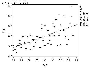
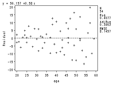
Fig. 10.1c, p. 406.
data temp;
  set temp;
  absr = abs(residual);
run;
symbol1 v=star h=.8;
axis1 order=(0 to 20 by 5);
proc gplot data = temp;
  plot absr*x/ vaxis = axis1;
run;
quit;
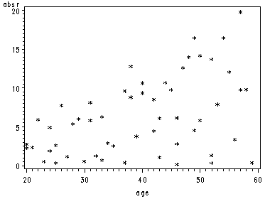
Regressing the absolute residuals against
X, formula 10.19 page 406.
proc reg data = temp ;
  model absr = x;
  output out = temp1 p = s ;
run;
quit;
The REG Procedure
Model: MODEL1
Dependent Variable: absrAnalysis of Variance
Sum of Mean
Source DF Squares Square F Value Pr > FModel 1 277.23091 277.23091 13.93 0.0005
Error 52 1034.62880 19.89671
Corrected Total 53 1311.85971Root MSE 4.46057 R-Square 0.2113
Dependent Mean 6.29301 Adj R-Sq 0.1962
Coeff Var 70.88141Parameter Estimates
Parameter Standard
Variable Label DF Estimate Error t Value Pr > |t|Intercept Intercept 1 -1.54948 2.18692 -0.71 0.4818
x age 1 0.19817 0.05309 3.73 0.0005
Obtaining the weights, w = 1/(s^2).
Table 10.1, p. 407.
data temp1;
  set temp1;
  w = 1/(s**2);
run;
proc print data = temp1 (obs = 10);
run;
Obs x y residual absr s w1 27 73 1.18224 1.18224 3.80117 0.06921
2 21 66 -2.33758 2.33758 2.61214 0.14656
3 22 63 -5.91761 5.91761 2.81031 0.12662
4 24 75 4.92233 4.92233 3.20666 0.09725
5 25 71 0.34230 0.34230 3.40483 0.08626
6 23 70 0.50236 0.50236 3.00849 0.11049
7 20 65 -2.75755 2.75755 2.41397 0.17161
8 20 70 2.24245 2.24245 2.41397 0.17161
9 29 79 6.02218 6.02218 4.19752 0.05676
10 24 72 1.92233 1.92233 3.20666 0.09725
The equation (10.20) by using WLS regression.
The option clb in the model statement supplies the confidence interval for the parameters.
proc reg data = temp1;
  weight w;
  model y = x / clb;
run;
quit;
The REG Procedure
Model: MODEL1
Dependent Variable: y DbpWeight: w
Analysis of Variance
Sum of Mean
Source DF Squares Square F Value Pr > FModel 1 83.34082 83.34082 56.64 <.0001
Error 52 76.51351 1.47141
Corrected Total 53 159.85432Root MSE 1.21302 R-Square 0.5214
Dependent Mean 73.55134 Adj R-Sq 0.5122
Coeff Var 1.64921Parameter Estimates
Parameter Standard
Variable Label DF Estimate Error t Value Pr > |t| 95% Confidence LimitsIntercept Intercept 1 55.56577 2.52092 22.04 <.0001 50.50718 60.62436
x age 1 0.59634 0.07924 7.53 <.0001 0.43734 0.75534
Inputting data for Ridge Regression example, p. 413.
data ch7tab01;
  input X1 X2 X3 Y;
  label x1 = 'Triceps'
        x2 = 'Thigh cir.'
	x3 = 'Midarm cir.'
         y = 'body fat';
  cards;
  19.5  43.1  29.1  11.9
  24.7  49.8  28.2  22.8
  30.7  51.9  37.0  18.7
  29.8  54.3  31.1  20.1
  19.1  42.2  30.9  12.9
  25.6  53.9  23.7  21.7
  31.4  58.5  27.6  27.1
  27.9  52.1  30.6  25.4
  22.1  49.9  23.2  21.3
  25.5  53.5  24.8  19.3
  31.1  56.6  30.0  25.4
  30.4  56.7  28.3  27.2
  18.7  46.5  23.0  11.7
  19.7  44.2  28.6  17.8
  14.6  42.7  21.3  12.8
  29.5  54.4  30.1  23.9
  27.7  55.3  25.7  22.6
  30.2  58.6  24.6  25.4
  22.7  48.2  27.1  14.8
  25.2  51.0  27.5  21.1
;
run;
Transforming the variables using the correlation transformation (7.44).
proc sql;
  create table ch7tab1a as
  select *, ( y - mean(y) )/( std(y)*( sqrt( count(y)-1 ) ) ) as ty,
            ( x1 - mean(x1) )/( std(x1)*( sqrt( count(x1)-1 ) ) ) as tx1,
	    ( x2 - mean(x2) )/( std(x2)*( sqrt( count(x2)-1 ) ) ) as tx2,
	    ( x3 - mean(x3) )/( std(x3)*( sqrt( count(x3)-1 ) ) ) as tx3
  from ch7tab01;
quit;
Ridge Regression on Body fat data.
Fig. 10.3, p. 413.
symbol1 v=dot h=.8;
proc reg data = ch7tab1a outest = temp outstb noprint;
  model y = x1-x3/ ridge = (0.001 to 0.1 by .001) outvif  ;
  plot / ridgeplot vref=0;
run;
quit;
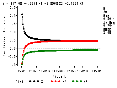
The equations at the bottom of p. 413.
The first line are the coefficients for the original variables and the second line
are the coefficients for the transformed variables. The transformation shown in (7.44)
is done automatically by SAS so there is no need to manually transform the variables
yourself. Notice that we used the untransformed variables in the regression models!
proc reg data = ch7tab1a outest = temp outstb noprint;
  model y = x1-x3 / ridge = 0.02;
run;
quit;
proc print data = temp;
  where _ridge_ = 0.02 and y = -1;
  var y intercept x1 x2 x3;
run;
Obs Y Intercept X1 X2 X32 -1 -7.40343 0.55535 0.36814 -0.19163
3 -1 0.00000 0.54633 0.37740 -0.13687
Table 10.2, p. 414.
The outstb option in the proc statement tells SAS to put the parameter estimates in the
output temp1. These can then be chosen by specifying RIDGESTB in the where statement of
the proc print.
proc reg data = ch7tab1a outest = temp outstb  outvif;
  model y = x1-x3/ridge = (0.0 to 0.01 by 0.002 0.02 to 0.05 by 0.01 0.5 1.0);
run;quit;
proc print data = temp;
  where _type_ = 'RIDGESTB';
  var _ridge_ x1 x2 x3;
run;
The REG Procedure
Model: MODEL1
Dependent Variable: Y body fatAnalysis of Variance
Sum of Mean
Source DF Squares Square F Value Pr > FModel 3 396.98461 132.32820 21.52 <.0001
Error 16 98.40489 6.15031
Corrected Total 19 495.38950Root MSE 2.47998 R-Square 0.8014
Dependent Mean 20.19500 Adj R-Sq 0.7641
Coeff Var 12.28017Parameter Estimates
Parameter Standard
Variable Label DF Estimate Error t Value Pr > |t|Intercept Intercept 1 117.08469 99.78240 1.17 0.2578
X1 Triceps 1 4.33409 3.01551 1.44 0.1699
X2 Thigh cir. 1 -2.85685 2.58202 -1.11 0.2849
X3 Midarm cir. 1 -2.18606 1.59550 -1.37 0.1896
Obs _RIDGE_ X1 X2 X34 0.000 4.26370 -2.92870 -1.56142
7 0.002 1.44066 -0.41129 -0.48127
10 0.004 1.00632 -0.02484 -0.31487
13 0.006 0.83002 0.13142 -0.24716
16 0.008 0.73433 0.21576 -0.21030
19 0.010 0.67417 0.26841 -0.18703
22 0.020 0.54633 0.37740 -0.13687
25 0.030 0.50038 0.41341 -0.11808
28 0.040 0.47600 0.43024 -0.10758
31 0.050 0.46046 0.43924 -0.10051
34 0.500 0.33772 0.37906 -0.02950
37 1.000 0.27977 0.31007 -0.00594
Table 10.3, p. 414.
The outvif option in the proc statement of the regression tells SAS to put the VIF’s
in the output temp1. These can then be chosen by specifying RIDGEVIF in the where
statement of the proc print.
proc print data = temp;
  where _type_ = 'RIDGEVIF';
  var _ridge_ x1 x2 x3;
run;
Obs _RIDGE_ X1 X2 X32 0.000 708.843 564.343 104.606
5 0.002 50.559 40.448 8.280
8 0.004 16.982 13.725 3.363
11 0.006 8.503 6.976 2.119
14 0.008 5.147 4.305 1.624
17 0.010 3.486 2.981 1.377
20 0.020 1.103 1.081 1.011
23 0.030 0.626 0.697 0.923
26 0.040 0.453 0.555 0.881
29 0.050 0.370 0.486 0.853
32 0.500 0.154 0.214 0.403
35 1.000 0.107 0.136 0.227
Inputting the Mathematics Proficiency Data, Table 10.4, p. 421.
Note: The easiest method of including observations with multiple words in one string
variable is to connect the words with an underscore.
data ch10tab11;
  input state $ y x1 x2 x3 x4 x5;
  label y = 'Math profeciency'
        x1 = 'Parents'
        x2 = 'Homelib'
        x3 = 'Reading'
        x4 = 'TV Watching'
        x5 = 'Absences';
cards;
 Alabama                 252  75  78  34  18  18
 Arizona                 259  75  73  41  12  26
 Arkansas                256  77  77  28  20  23
 California              256  78  68  42  11  28
 Colorado                267  78  85  38   9  25
 Connecticut             270  79  86  43  12  22
 Delaware                261  75  83  32  18  28
 Distric_of_Columbia     231  47  76  24  33  37
 Florida                 255  75  73  31  19  27
 Georgia                 258  73  80  36  17  22
 Guam                    231  81  64  32  20  28
 Hawaii                  251  78  69  36  23  26
 Idaho                   272  84  84  48   7  21
 Illinois                260  78  82  43  14  21
 Indiana                 267  81  84  37  11  23
 Iowa                    278  83  88  43   8  20
 Kentucky                256  79  78  36  14  23
 Louisiana               246  73  76  36  19  27
 Maryland                260  75  83  34  19  27
 Michigan                264  77  84  31  14  25
 Minnesota               276  83  88  36   7  20
 Montana                 280  83  88  44   6  21
 Nebraska                276  85  88  42   9  19
 New_Hampshire           273  83  88  40   7  22
 New_Jersey              269  79  84  41  13  23
 New_Mexico              256  77  72  40  11  27
 New_York                261  76  79  35  17  29
 North_Carolina          250  74  78  37  21  25
 North_Dakota            281  85  90  41   6  14
 Ohio                    264  79  84  36  11  22
 Oklahoma                263  78  78  37  14  22
 Oregon                  271  81  82  41   9  31
 Pennsylvania            266  80  86  34  10  24
 Rhode_Island            260  78  80  38  12  28
 Texas                   258  77  70  34  15  18
 Virgin_Islands          218  63  76  23  27  22
 Virginia                264  78  82  33  16  24
 West_Virginia           256  82  80  36  16  25
 Wisconsin               274  81  86  38   8  21
 Wyoming                 272  85  86  43   7  23
;
run;
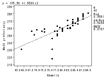
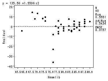
Fig. 10.5, p. 421.
proc reg data = ch10tab11;
  model y = x2;
  plot y*x2 r.*x2;
run;
quit;
The REG Procedure
Model: MODEL1
Dependent Variable: y Math profeciencyAnalysis of Variance
Sum of Mean
Source DF Squares Square F Value Pr > FModel 1 3769.30965 3769.30965 47.42 <.0001
Error 38 3020.59035 79.48922
Corrected Total 39 6789.90000Root MSE 8.91567 R-Square 0.5551
Dependent Mean 260.95000 Adj R-Sq 0.5434
Coeff Var 3.41662Parameter Estimates
Parameter Standard
Variable Label DF Estimate Error t Value Pr > |t|Intercept Intercept 1 135.55589 18.26408 7.42 <.0001
x2 Homelib 1 1.55963 0.22649 6.89 <.0001
The model using robust regression.
Invoking the macro robust_hubert which in turn invokes the mad macro. It will create
two pictures but this can be modified. We show the Predicted by Residual below.
%include 'c:neter/sas/examples/alsm/mad.sas';
%include 'c:neter/sas/examples/alsm/robust_hubert.sas';
%robust_hubert(ch10tab11, y, x2, 0.000005, 8);
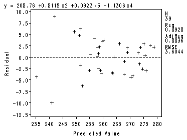
Below you can see the results of the OLS fit (10.49, page 422) followed by the iterations
of the reweighted least squares (see table 10.5, page 422) and then the final results (see 10.51, page 423).
The REG Procedure
Model: MODEL1
Dependent Variable: y Math profeciencyAnalysis of Variance
Sum of Mean
Source DF Squares Square F Value Pr > FModel 1 3769.30965 3769.30965 47.42 <.0001
Error 38 3020.59035 79.48922
Corrected Total 39 6789.90000Root MSE 8.91567 R-Square 0.5551
Dependent Mean 260.95000 Adj R-Sq 0.5434
Coeff Var 3.41662Parameter Estimates
Parameter Standard
Variable Label DF Estimate Error t Value Pr > |t|Intercept Intercept 1 135.55589 18.26408 7.42 <.0001
x2 Homelib 1 1.55963 0.22649 6.89 <.0001
Obs r u _w2_1 -5.2069 -0.77336 1.00000
2 9.5912 1.42455 0.94416
3 0.3527 0.05239 1.00000
4 14.3894 2.13719 0.62933
5 -1.1243 -0.16699 1.00000
6 0.3161 0.04695 1.00000
7 -4.0050 -0.59485 1.00000
8 -23.0876 -3.42911 0.39223
9 5.5912 0.83044 1.00000
10 -2.3261 -0.34549 1.00000
Obs r _w2_1 -6.1773 1.00000
2 8.3454 1.00000
3 -0.6728 1.00000
4 12.8681 0.70085
5 -1.7091 1.00000
6 -0.2136 1.00000
7 -4.7000 1.00000
8 -24.1682 0.37316
9 4.3454 1.00000
10 -3.1864 1.00000
Obs r _w2_1 -6.3179 1.00000
2 8.1025 1.00000
3 -0.8338 1.00000
4 12.5230 0.70388
5 -1.7065 1.00000
6 -0.1906 1.00000
7 -4.7384 1.00000
8 -24.3498 0.36200
9 4.1025 1.00000
10 -3.2861 1.00000
Obs r _w2_1 -6.3529 1.00000
2 8.0501 1.00000
3 -0.8723 1.00000
4 12.4531 0.70504
5 -1.7171 1.00000
6 -0.1977 1.00000
7 -4.7559 1.00000
8 -24.3917 0.35995
9 4.0501 1.00000
10 -3.3141 1.00000
Obs r _w2_1 -6.3602 1.00000
2 8.0389 1.00000
3 -0.8804 1.00000
4 12.4380 0.70527
5 -1.7190 1.00000
6 -0.1988 1.00000
7 -4.7593 1.00000
8 -24.4006 0.35951
9 4.0389 1.00000
10 -3.3198 1.00000
Obs r _w2_1 -6.3618 1.00000
2 8.0365 1.00000
3 -0.8821 1.00000
4 12.4348 0.70532
5 -1.7194 1.00000
6 -0.1990 1.00000
7 -4.7600 1.00000
8 -24.4025 0.35941
9 4.0365 1.00000
10 -3.3211 1.00000
Obs r _w2_1 -6.3621 1.00000
2 8.0360 1.00000
3 -0.8825 1.00000
4 12.4341 0.70533
5 -1.7194 1.00000
6 -0.1991 1.00000
7 -4.7602 1.00000
8 -24.4029 0.35939
9 4.0360 1.00000
10 -3.3213 1.00000
Obs r _w2_1 -6.3622 1.00000
2 8.0359 1.00000
3 -0.8826 1.00000
4 12.4340 0.70533
5 -1.7195 1.00000
6 -0.1991 1.00000
7 -4.7602 1.00000
8 -24.4029 0.35939
9 4.0359 1.00000
10 -3.3214 1.00000The REG Procedure
Model: MODEL1
Dependent Variable: y Math profeciencyWeight: _w2_
Analysis of Variance
Sum of Mean
Source DF Squares Square F Value Pr > FModel 1 3165.87899 3165.87899 78.49 <.0001
Error 38 1532.63864 40.33260
Corrected Total 39 4698.51763Root MSE 6.35079 R-Square 0.6738
Dependent Mean 262.40346 Adj R-Sq 0.6652
Coeff Var 2.42024Parameter Estimates
Parameter Standard
Variable Label DF Estimate Error t Value Pr > |t|Intercept Intercept 1 142.95244 13.52182 10.57 <.0001
x2 Homelib 1 1.47961 0.16700 8.86 <.0001
Sections 10.4 and 10.5 were skipped. For help using Loess method please come see us in
consulting and for Bootstrapping you might consider using the bs command in Stata, for example
https://stats.idre.ucla.edu/stat/stata/examples/ara/arastata16.htm.
Section 10.6–Model Validation!
Inputting the Surgical Unit data, Table 8.1, p. 335.
data ch8tab01;
  input x1 x2 x3 x4 y logy;
  label x1 = 'blood-clotting'
        x2 = 'prognostic'
	x3 = 'enzyme'
	x4 = 'liver function'
	 y = 'survival'
      logy = 'Logsurvival';
cards;
   6.7  62   81  2.59  200  2.3010
   5.1  59   66  1.70  101  2.0043
   7.4  57   83  2.16  204  2.3096
   6.5  73   41  2.01  101  2.0043
   7.8  65  115  4.30  509  2.7067
   5.8  38   72  1.42   80  1.9031
   5.7  46   63  1.91   80  1.9031
   3.7  68   81  2.57  127  2.1038
   6.0  67   93  2.50  202  2.3054
   3.7  76   94  2.40  203  2.3075
   6.3  84   83  4.13  329  2.5172
   6.7  51   43  1.86   65  1.8129
   5.8  96  114  3.95  830  2.9191
   5.8  83   88  3.95  330  2.5185
   7.7  62   67  3.40  168  2.2253
   7.4  74   68  2.40  217  2.3365
   6.0  85   28  2.98   87  1.9395
   3.7  51   41  1.55   34  1.5315
   7.3  68   74  3.56  215  2.3324
   5.6  57   87  3.02  172  2.2355
   5.2  52   76  2.85  109  2.0374
   3.4  83   53  1.12  136  2.1335
   6.7  26   68  2.10   70  1.8451
   5.8  67   86  3.40  220  2.3424
   6.3  59  100  2.95  276  2.4409
   5.8  61   73  3.50  144  2.1584
   5.2  52   86  2.45  181  2.2577
  11.2  76   90  5.59  574  2.7589
   5.2  54   56  2.71   72  1.8573
   5.8  76   59  2.58  178  2.2504
   3.2  64   65  0.74   71  1.8513
   8.7  45   23  2.52   58  1.7634
   5.0  59   73  3.50  116  2.0645
   5.8  72   93  3.30  295  2.4698
   5.4  58   70  2.64  115  2.0607
   5.3  51   99  2.60  184  2.2648
   2.6  74   86  2.05  118  2.0719
   4.3   8  119  2.85  120  2.0792
   4.8  61   76  2.45  151  2.1790
   5.4  52   88  1.81  148  2.1703
   5.2  49   72  1.84   95  1.9777
   3.6  28   99  1.30   75  1.8751
   8.8  86   88  6.40  483  2.6840
   6.5  56   77  2.85  153  2.1847
   3.4  77   93  1.48  191  2.2810
   6.5  40   84  3.00  123  2.0899
   4.5  73  106  3.05  311  2.4928
   4.8  86  101  4.10  398  2.5999
   5.1  67   77  2.86  158  2.1987
   3.9  82  103  4.55  310  2.4914
   6.6  77   46  1.95  124  2.0934
   6.4  85   40  1.21  125  2.0969
   6.4  59   85  2.33  198  2.2967
   8.8  78   72  3.20  313  2.4955
;
run;
Inputting the Validation dataset, Table 10.10, p. 439.
data ch10tab10;
 input x1 x2 x3 x4 logy;
 label x1 = 'Clotting'
       x2 = 'Prognostic'
       x3 = 'Enzyme'
       x4 = 'Liver'
     logy = 'logSurvival';
cards;
   7.1  23   78  1.93  2.0326
   4.9  66   91  3.05  2.4086
   6.4  90   35  1.06  2.2177
   5.7  35   70  2.13  1.9078
   6.1  42   69  2.25  2.0035
   8.0  27   83  2.03  2.0945
   6.8  34   51  1.27  1.7652
   4.7  63   36  1.71  1.7925
   7.0  47   67  1.60  2.1292
   6.7  69   65  2.91  2.2295
   6.7  46   78  3.26  2.1524
   5.8  60   86  3.11  2.3188
   6.7  56   32  1.53  1.9039
   6.8  51   58  2.18  2.0508
   7.2  95   82  4.68  2.6525
   7.4  52   67  3.28  2.2053
   5.3  53   62  2.42  1.9246
   3.5  58   84  1.74  2.1541
   6.8  74   79  2.25  2.4970
   4.4  47   49  2.42  1.7237
   7.0  66  118  4.69  2.8339
   6.7  61   57  3.87  2.1282
   5.6  75  103  3.11  2.6884
   6.9  58   88  3.46  2.4284
   6.2  62   57  1.25  2.0261
   4.7  97   27  1.77  2.0843
   6.8  69   60  2.90  2.2826
   6.0  73   58  1.22  2.2073
   5.9  50   62  3.19  2.0443
   5.5  88   74  3.21  2.4863
   3.8  55   52  1.41  1.9037
   4.3  99   83  3.93  2.6647
   6.6  48   54  2.94  1.9071
   6.2  42   63  1.85  1.9093
   5.0  60  105  3.17  2.4389
   5.8  62   82  3.18  2.3343
   4.7  42   10  0.28  1.3379
   5.7  70   59  2.28  2.1996
   4.7  64   48  1.30  1.8795
   7.8  74   40  2.58  2.1504
   2.9  43   32  0.94  1.4330
   4.9  72   90  3.51  2.4381
   4.6  73   57  2.82  2.1075
   5.9  78   70  4.28  2.2843
   4.6  69   70  3.17  2.1615
   6.1  53   52  1.84  2.0558
   5.9  88   98  3.33  2.7249
   4.7  66   68  1.80  2.0520
  10.4  62   85  4.65  2.6810
   5.8  70   64  2.52  2.2604
   5.4  64   81  1.36  2.2553
   6.9  90   33  2.78  2.1745
   7.9  45   55  2.46  2.0224
   4.5  68   60  2.07  2.1413

;;;
run;
Table 10.9, p. 438.
proc reg data = ch8tab01 outest = temp;
  title 'Results from the Model Building Data set';
  model logy = x1 x2 x3/press;
run;
quit;
proc print data = temp;
 var _press_;
run;
proc reg data = ch10tab10 outest = temp;
  title 'Results from the Validation Data set';
  model logy = x1 x2 x3/ press;
run;
quit;
proc print data = temp;
 var _press_;
run;
title ;
Results from the Model Building Data set
The REG Procedure
Model: MODEL1
Dependent Variable: logy LogsurvivalAnalysis of Variance
Sum of Mean
Source DF Squares Square F Value Pr > FModel 3 3.86291 1.28764 586.04 <.0001
Error 50 0.10986 0.00220
Corrected Total 53 3.97277Root MSE 0.04687 R-Square 0.9723
Dependent Mean 2.20614 Adj R-Sq 0.9707
Coeff Var 2.12470Parameter Estimates
Parameter Standard
Variable Label DF Estimate Error t Value Pr > |t|Intercept Intercept 1 0.48362 0.04263 11.34 <.0001
x1 blood-clotting 1 0.06923 0.00408 16.98 <.0001
x2 prognostic 1 0.00929 0.00038250 24.30 <.0001
x3 enzyme 1 0.00952 0.00030641 31.08 <.0001
Results from the Model Building Data set
Obs _PRESS_1 0.14045
Results from the Validation Data set
The REG Procedure
Model: MODEL1
Dependent Variable: logy logSurvivalAnalysis of Variance
Sum of Mean
Source DF Squares Square F Value Pr > FModel 3 4.62507 1.54169 730.29 <.0001
Error 50 0.10555 0.00211
Corrected Total 53 4.73062Root MSE 0.04595 R-Square 0.9777
Dependent Mean 2.16466 Adj R-Sq 0.9763
Coeff Var 2.12257Parameter Estimates
Parameter Standard
Variable Label DF Estimate Error t Value Pr > |t|Intercept Intercept 1 0.50082 0.04192 11.95 <.0001
x1 Clotting 1 0.06741 0.00498 13.53 <.0001
x2 Prognostic 1 0.01011 0.00037193 27.18 <.0001
x3 Enzyme 1 0.00974 0.00030225 32.22 <.0001
Results from the Validation Data set
Obs _PRESS_1 0.12125
Case Example–Mathematical Proficiency.
Note: This data has already been input in this program.
Fig. 10.10a, p. 441.
Calling the scatter matrix macro.
%include 'c:neter/sas/examples/alsm/scatter.sas';
%scatter(data = ch10tab11, var= y x1 x2 x3 x4 x5);
<The scatterplot is not shown>
Fig. 10.10b, p. 441.
proc corr data = ch10tab11;
  var y x1-x5;
run;
he CORR Procedure6 Variables: y x1 x2 x3 x4 x5
Simple Statistics
Variable N Mean Std Dev Sum Minimum Maximum Label
y 40 260.95000 13.19470 10438 218.00000 281.00000 Math profeciency
x1 40 77.70000 6.49339 3108 47.00000 85.00000 Parents
x2 40 80.40000 6.30344 3216 64.00000 90.00000 Homelib
x3 40 36.85000 5.26016 1474 23.00000 48.00000 Reading
x4 40 14.00000 5.99572 560.00000 6.00000 33.00000 TV Watching
x5 40 23.92500 4.07863 957.00000 14.00000 37.00000 AbsencesPearson Correlation Coefficients, N = 40
Prob > |r| under H0: Rho=0y x1 x2 x3 x4 x5
y 1.00000 0.74141 0.74507 0.71659 -0.87348 -0.48034
Math profeciency <.0001 <.0001 <.0001 <.0001 0.0017x1 0.74141 1.00000 0.39454 0.69304 -0.83115 -0.56531
Parents <.0001 0.0118 <.0001 <.0001 0.0001x2 0.74507 0.39454 1.00000 0.37692 -0.59364 -0.44262
Homelib <.0001 0.0118 0.0165 <.0001 0.0042x3 0.71659 0.69304 0.37692 1.00000 -0.79187 -0.35669
Reading <.0001 <.0001 0.0165 <.0001 0.0239x4 -0.87348 -0.83115 -0.59364 -0.79187 1.00000 0.51168
TV Watching <.0001 <.0001 <.0001 <.0001 0.0007x5 -0.48034 -0.56531 -0.44262 -0.35669 0.51168 1.00000
Absences 0.0017 0.0001 0.0042 0.0239 0.0007
Fitted model (10.61) p. 441.
proc reg data = ch10tab11;
  model y = x1-x5;
  output out = temp h = hii student=ti cookd = Di;
run;
quit;
The REG Procedure
Model: MODEL1
Dependent Variable: y Math profeciencyAnalysis of Variance
Sum of Mean
Source DF Squares Square F Value Pr > FModel 5 5846.32774 1169.26555 42.13 <.0001
Error 34 943.57226 27.75213
Corrected Total 39 6789.90000Root MSE 5.26803 R-Square 0.8610
Dependent Mean 260.95000 Adj R-Sq 0.8406
Coeff Var 2.01879Parameter Estimates
Parameter Standard
Variable Label DF Estimate Error t Value Pr > |t|Intercept Intercept 1 155.03039 36.23830 4.28 0.0001
x1 Parents 1 0.39115 0.25709 1.52 0.1374
x2 Homelib 1 0.86387 0.17971 4.81 <.0001
x3 Reading 1 0.36162 0.26896 1.34 0.1877
x4 TV Watching 1 -0.84672 0.35254 -2.40 0.0219
x5 Absences 1 0.19229 0.26361 0.73 0.4707
Table 10.12, p. 442.
proc print data = temp (obs = 10);
 var hii ti Di;
run;
Obs hii ti Di1 0.16014 -0.05464 0.00009
2 0.18531 0.40076 0.00609
3 0.16201 1.39338 0.06256
4 0.29069 0.10337 0.00073
5 0.09541 -0.57826 0.00588
6 0.12133 0.03171 0.00002
7 0.11685 0.64985 0.00931
8 0.69026 1.39145 0.71914
9 0.09109 1.44485 0.03487
10 0.07670 0.48432 0.00325
The fitted model using robust regression (10.62), p. 442.
Running the Hubert robust regression.
Running the Hubert/Biweight robust regression which is similar to rreg in Stata.
Invoking two different macros.
Here is the first macro, robust_hubert.
%include 'c:neter/sas/examples/alsm/mad.sas';
%include 'c:neter/sas/examples/alsm/robust_hubert.sas';
%robust_hubert(ch10tab11, y, x2 x3 x4, 0.0005, 9);
The REG Procedure
Model: MODEL1
Dependent Variable: y Math profeciencyAnalysis of Variance
Sum of Mean
Source DF Squares Square F Value Pr > FModel 3 5781.00353 1927.00118 68.76 <.0001
Error 36 1008.89647 28.02490
Corrected Total 39 6789.90000Root MSE 5.29386 R-Square 0.8514
Dependent Mean 260.95000 Adj R-Sq 0.8390
Coeff Var 2.02869Parameter Estimates
Parameter Standard
Variable Label DF Estimate Error t Value Pr > |t|Intercept Intercept 1 199.61074 21.52892 9.27 <.0001
x2 Homelib 1 0.78043 0.17020 4.59 <.0001
x3 Reading 1 0.40118 0.26876 1.49 0.1442
x4 TV Watching 1 -1.15647 0.27140 -4.26 0.0001
Obs r u _w2_1 -1.30771 -0.28443 1.00000
2 -0.15269 -0.03321 1.00000
3 8.19275 1.78192 0.75481
4 -0.80821 -0.17578 1.00000
5 -3.78369 -0.82295 1.00000
6 -0.10060 -0.02188 1.00000
7 4.59251 0.99887 1.00000
8 0.61205 0.13312 1.00000
9 7.95444 1.73008 0.77742
10 1.17259 0.25504 1.00000
Obs r _w2_1 -1.97842 1.00000
2 0.70596 1.00000
3 6.47543 0.92592
4 0.45509 1.00000
5 -3.93974 1.00000
6 0.55384 1.00000
7 3.35113 1.00000
8 -1.92494 1.00000
9 6.95415 0.86218
10 0.78291 1.00000
Obs r _w2_1 -2.16585 1.00000
2 0.68042 1.00000
3 6.05663 0.99024
4 0.40731 1.00000
5 -4.00323 1.00000
6 0.74252 1.00000
7 3.13259 1.00000
8 -2.35721 1.00000
9 6.60526 0.90799
10 0.68544 1.00000
Obs r _w2_1 -2.24010 1.00000
2 0.60703 1.00000
3 5.90929 1.00000
4 0.29252 1.00000
5 -4.02355 1.00000
6 0.81795 1.00000
7 3.07963 1.00000
8 -2.47327 1.00000
9 6.45193 0.93764
10 0.64893 1.00000
Obs r _w2_1 -2.26999 1.00000
2 0.55502 1.00000
3 5.85944 1.00000
4 0.21310 1.00000
5 -4.02818 1.00000
6 0.84502 1.00000
7 3.07071 1.00000
8 -2.50289 1.00000
9 6.38705 0.94683
10 0.63394 1.00000
Obs r _w2_1 -2.28228 1.00000
2 0.53287 1.00000
3 5.83868 1.00000
4 0.17892 1.00000
5 -4.02932 1.00000
6 0.85736 1.00000
7 3.06771 1.00000
8 -2.51505 1.00000
9 6.35958 0.95076
10 0.62809 1.00000
Obs r _w2_1 -2.28754 1.00000
2 0.52337 1.00000
3 5.82983 1.00000
4 0.16428 1.00000
5 -4.02981 1.00000
6 0.86264 1.00000
7 3.06644 1.00000
8 -2.52021 1.00000
9 6.34783 0.95245
10 0.62559 1.00000
Obs r _w2_1 -2.28978 1.00000
2 0.51931 1.00000
3 5.82603 1.00000
4 0.15802 1.00000
5 -4.03002 1.00000
6 0.86489 1.00000
7 3.06590 1.00000
8 -2.52242 1.00000
9 6.34281 0.95317
10 0.62453 1.00000
Obs r _w2_1 -2.29074 1.00000
2 0.51758 1.00000
3 5.82441 1.00000
4 0.15534 1.00000
5 -4.03011 1.00000
6 0.86586 1.00000
7 3.06567 1.00000
8 -2.52337 1.00000
9 6.34066 0.95348
10 0.62407 1.00000The REG Procedure
Model: MODEL1
Dependent Variable: y Math profeciencyWeight: _w2_
Analysis of Variance
Sum of Mean
Source DF Squares Square F Value Pr > FModel 3 4391.06625 1463.68875 83.27 <.0001
Error 36 632.76457 17.57679
Corrected Total 39 5023.83082Root MSE 4.19247 R-Square 0.8740
Dependent Mean 262.15459 Adj R-Sq 0.8636
Coeff Var 1.59924Parameter Estimates
Parameter Standard
Variable Label DF Estimate Error t Value Pr > |t|Intercept Intercept 1 207.83984 17.58882 11.82 <.0001
x2 Homelib 1 0.79410 0.14083 5.64 <.0001
x3 Reading 1 0.16362 0.22036 0.74 0.4626
x4 TV Watching 1 -1.16953 0.21890 -5.34 <.0001
Here is the second macro, robust_hb.
%include 'c:neter/sas/examples/alsm/robust_hb.sas';
%robust_hb(ch10tab11, y, x2 x3 x4, 0.01, 0.0005, 9);
The REG Procedure
Model: MODEL1
Dependent Variable: y Math profeciencyAnalysis of Variance
Sum of Mean
Source DF Squares Square F Value Pr > FModel 3 5781.00353 1927.00118 68.76 <.0001
Error 36 1008.89647 28.02490
Corrected Total 39 6789.90000Root MSE 5.29386 R-Square 0.8514
Dependent Mean 260.95000 Adj R-Sq 0.8390
Coeff Var 2.02869Parameter Estimates
Parameter Standard
Variable Label DF Estimate Error t Value Pr > |t|Intercept Intercept 1 199.61074 21.52892 9.27 <.0001
x2 Homelib 1 0.78043 0.17020 4.59 <.0001
x3 Reading 1 0.40118 0.26876 1.49 0.1442
x4 TV Watching 1 -1.15647 0.27140 -4.26 0.0001
Obs r u _w2_1 -1.30771 -0.28443 1.00000
2 -0.15269 -0.03321 1.00000
3 8.19275 1.78192 0.75481
4 -0.80821 -0.17578 1.00000
5 -3.78369 -0.82295 1.00000
6 -0.10060 -0.02188 1.00000
7 4.59251 0.99887 1.00000
8 0.61205 0.13312 1.00000
9 7.95444 1.73008 0.77742
10 1.17259 0.25504 1.00000
Obs r _w2_1 -1.97842 1.00000
2 0.70596 1.00000
3 6.47543 0.92592
4 0.45509 1.00000
5 -3.93974 1.00000
6 0.55384 1.00000
7 3.35113 1.00000
8 -1.92494 1.00000
9 6.95415 0.86218
10 0.78291 1.00000
Obs r _w2_1 -2.16585 1.00000
2 0.68042 1.00000
3 6.05663 0.99024
4 0.40731 1.00000
5 -4.00323 1.00000
6 0.74252 1.00000
7 3.13259 1.00000
8 -2.35721 1.00000
9 6.60526 0.90799
10 0.68544 1.00000
Obs r _w2_1 -2.24010 1.00000
2 0.60703 1.00000
3 5.90929 1.00000
4 0.29252 1.00000
5 -4.02355 1.00000
6 0.81795 1.00000
7 3.07963 1.00000
8 -2.47327 1.00000
9 6.45193 0.93764
10 0.64893 1.00000
Obs r _w2_1 -2.26999 1.00000
2 0.55502 1.00000
3 5.85944 1.00000
4 0.21310 1.00000
5 -4.02818 1.00000
6 0.84502 1.00000
7 3.07071 1.00000
8 -2.50289 1.00000
9 6.38705 0.94683
10 0.63394 1.00000
Obs r _w2_1 -2.28228 1.00000
2 0.53287 1.00000
3 5.83868 1.00000
4 0.17892 1.00000
5 -4.02932 1.00000
6 0.85736 1.00000
7 3.06771 1.00000
8 -2.51505 1.00000
9 6.35958 0.95076
10 0.62809 1.00000
Obs r _w2_1 -2.28754 1.00000
2 0.52337 1.00000
3 5.82983 1.00000
4 0.16428 1.00000
5 -4.02981 1.00000
6 0.86264 1.00000
7 3.06644 1.00000
8 -2.52021 1.00000
9 6.34783 0.95245
10 0.62559 1.00000
Obs r _w2_1 -2.28978 0.97649
2 0.51931 0.99878
3 5.82603 0.85279
4 0.15802 0.99989
5 -4.03002 0.92810
6 0.86489 0.99663
7 3.06590 0.95806
8 -2.52242 0.97151
9 6.34281 0.82680
10 0.62453 0.99824
Obs r _w2_1 -2.73012 0.96699
2 0.86459 0.99666
3 4.96329 0.89302
4 0.72986 0.99762
5 -4.06566 0.92755
6 1.00401 0.99550
7 2.37379 0.97500
8 -4.09078 0.92667
9 5.80575 0.85515
10 0.29495 0.99961
Obs r _w2_1 -2.81014 0.96404
2 0.83110 0.99683
3 4.83738 0.89535
4 0.68947 0.99782
5 -4.06672 0.92544
6 1.02494 0.99518
7 2.29836 0.97587
8 -4.29038 0.91720
9 5.68803 0.85684
10 0.23689 0.99974
Obs r _w2_1 -2.83138 0.96315
2 0.80418 0.99700
3 4.80324 0.89581
4 0.64927 0.99804
5 -4.06725 0.92471
6 1.03939 0.99499
7 2.28767 0.97586
8 -4.32471 0.91509
9 5.64737 0.85748
10 0.22449 0.99977
Obs r _w2_1 -2.83871 0.96282
2 0.79223 0.99708
3 4.79108 0.89594
4 0.63096 0.99815
5 -4.06757 0.92442
6 1.04606 0.99491
7 2.28533 0.97582
8 -4.33367 0.91444
9 5.63172 0.85773
10 0.22075 0.99977
Obs r _w2_1 -2.84151 0.96269
2 0.78734 0.99711
3 4.78636 0.89600
4 0.62341 0.99819
5 -4.06772 0.92431
6 1.04886 0.99488
7 2.28460 0.97580
8 -4.33669 0.91420
9 5.62552 0.85783
10 0.21941 0.99978
Obs r _w2_1 -2.84261 0.96264
2 0.78538 0.99712
3 4.78449 0.89602
4 0.62036 0.99820
5 -4.06779 0.92426
6 1.05000 0.99486
7 2.28434 0.97579
8 -4.33783 0.91411
9 5.62305 0.85788
10 0.21890 0.99978
Obs r _w2_1 -2.84305 0.96262
2 0.78459 0.99713
3 4.78374 0.89602
4 0.61914 0.99821
5 -4.06782 0.92425
6 1.05046 0.99486
7 2.28423 0.97579
8 -4.33828 0.91407
9 5.62206 0.85789
10 0.21869 0.99978The REG Procedure
Model: MODEL1
Dependent Variable: y Math profeciencyWeight: _w2_
Analysis of Variance
Sum of Mean
Source DF Squares Square F Value Pr > FModel 3 3786.64784 1262.21595 97.16 <.0001
Error 35 454.69842 12.99138
Corrected Total 38 4241.34626Root MSE 3.60436 R-Square 0.8928
Dependent Mean 262.64784 Adj R-Sq 0.8836
Coeff Var 1.37232Parameter Estimates
Parameter Standard
Variable Label DF Estimate Error t Value Pr > |t|Intercept Intercept 1 208.75986 15.50570 13.46 <.0001
x2 Homelib 1 0.81146 0.12370 6.56 <.0001
x3 Reading 1 0.09235 0.19497 0.47 0.6387
x4 TV Watching 1 -1.13056 0.19267 -5.87 <.0001
Fig. 10.11, p. 443.
proc reg data = ch10tab11;
  model y = x1-x5/ selection = rsquare best = 2 cp adjrsq ;
run;
quit;
The REG Procedure
Model: MODEL1
Dependent Variable: yR-Square Selection Method
Number in Adjusted
Model R-Square R-Square C(p) Variables in Model1 0.7630 0.7567 21.9929 x4
1 0.5551 0.5434 72.8418 x2
——————————————————————-
2 0.8422 0.8337 4.6039 x2 x4
2 0.7923 0.7810 16.8260 x1 x2
——————————————————————-
3 0.8514 0.8390 4.3538 x2 x3 x4
3 0.8507 0.8383 4.5237 x1 x2 x4
——————————————————————-
4 0.8589 0.8427 4.5321 x1 x2 x3 x4
4 0.8536 0.8369 5.8078 x1 x2 x4 x5
——————————————————————-
5 0.8610 0.8406 6.0000 x1 x2 x3 x4 x5
The model fitted by OLS (10.63), p. 443.
proc reg data = ch10tab11;
 model y = x2 x3 x4;
run;
quit;
The REG Procedure
Model: MODEL1
Dependent Variable: y Math profeciencyAnalysis of Variance
Sum of Mean
Source DF Squares Square F Value Pr > FModel 3 5781.00353 1927.00118 68.76 <.0001
Error 36 1008.89647 28.02490
Corrected Total 39 6789.90000Root MSE 5.29386 R-Square 0.8514
Dependent Mean 260.95000 Adj R-Sq 0.8390
Coeff Var 2.02869Parameter Estimates
Parameter Standard
Variable Label DF Estimate Error t Value Pr > |t|Intercept Intercept 1 199.61074 21.52892 9.27 <.0001
x2 Homelib 1 0.78043 0.17020 4.59 <.0001
x3 Reading 1 0.40118 0.26876 1.49 0.1442
x4 TV Watching 1 -1.15647 0.27140 -4.26 0.0001