Applied Linear Statistical Models by Neter, Kutner, et. al. Chapter 14: Logistic Regression, Poisson Regression and Generalized Linear Models

options nocenter nodate;

Inputting the Programming Task data, table 14.1, p. 576.

data ch14tab01;
  input x y ;
  label x = 'Experience'
        y = 'Success';
cards;
14  0  0.310262
29  0  0.835263
 6  0  0.109996
25  1  0.726602
18  1  0.461837
 4  0  0.082130
18  0  0.461837
12  0  0.245666
22  1  0.620812
 6  0  0.109996
30  1  0.856299
11  0  0.216980
30  1  0.856299
 5  0  0.095154
20  1  0.542404
13  0  0.276802
 9  0  0.167100
32  1  0.891664
24  0  0.693379
13  1  0.276802
19  0  0.502134
 4  0  0.082130
28  1  0.811825
22  1  0.620812
 8  1  0.145815
;
run;

Logistic Regression, table 14.1, p. 576.

proc logistic data = ch14tab01 descending;
  model y = x;
  output out = temp resdev=devresidual p = fittedp;
run;
proc print data = temp;
  var x y  fittedp devresidual;
run;

The LOGISTIC Procedure

Model Information

Data Set WORK.CH14TAB01
Response Variable y Success
Number of Response Levels 2
Number of Observations 25
Link Function Logit
Optimization Technique Fisher’s scoring

Response Profile

Ordered Total
Value y Frequency

1 1 11
2 0 14

Model Convergence Status

Convergence criterion (GCONV=1E-8) satisfied.

Model Fit Statistics

Intercept
Intercept and
Criterion Only Covariates

AIC 36.296 29.425
SC 37.515 31.862
-2 Log L 34.296 25.425

Testing Global Null Hypothesis: BETA=0

Test Chi-Square DF Pr > ChiSq

Likelihood Ratio 8.8719 1 0.0029
Score 7.9742 1 0.0047
Wald 6.1760 1 0.0129

Analysis of Maximum Likelihood Estimates

Standard
Parameter DF Estimate Error Chi-Square Pr > ChiSq

Intercept 1 -3.0597 1.2594 5.9029 0.0151
x 1 0.1615 0.0650 6.1760 0.0129

The LOGISTIC Procedure

Odds Ratio Estimates

Point 95% Wald
Effect Estimate Confidence Limits

x 1.175 1.035 1.335

Association of Predicted Probabilities and Observed Responses

Percent Concordant 82.5 Somers’ D 0.662
Percent Discordant 16.2 Gamma 0.671
Percent Tied 1.3 Tau-a 0.340
Pairs 154 c 0.831
Obs x y fittedp devresidual

1 14 0 0.31026 -0.86191
2 29 0 0.83526 -1.89916
3 6 0 0.11000 -0.48276
4 25 1 0.72660 0.79922
5 18 1 0.46184 1.24302
6 4 0 0.08213 -0.41400
7 18 0 0.46184 -1.11319
8 12 0 0.24567 -0.75089
9 22 1 0.62081 0.97645
10 6 0 0.11000 -0.48276
11 30 1 0.85630 0.55702
12 11 0 0.21698 -0.69942
13 30 1 0.85630 0.55702
14 5 0 0.09515 -0.44719
15 20 1 0.54240 1.10611
16 13 0 0.27680 -0.80507
17 9 0 0.16710 -0.60472
18 32 1 0.89166 0.47889
19 24 0 0.69338 -1.53762
20 13 1 0.27680 1.60278
21 19 0 0.50213 -1.18104
22 4 0 0.08213 -0.41400
23 28 1 0.81182 0.64571
24 22 1 0.62081 0.97645
25 8 1 0.14582 1.96235

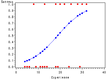
Fig. 14.3, p. 576.

proc sort data = temp;
  by x;
run;
goptions reset = all; 
symbol1 c=red v=dot h = .8 ;
symbol2 c=blue v=dot h=.8 i=join;
proc gplot data = temp;
  plot y*x fittedp*x / overlay;
run;
quit;
goptions reset = all;

Inputting Coupon Effectiveness data, Table 14.2, p. 579.

data ch14tab02;
  input x n r p;
  label x = 'Reduction'
        n = 'no.  households'
	r = 'coupons redeemed'
	p = 'proportion of coupons redeemed';
cards;
   5  200   30  .150
  10  200   55  .275
  15  200   70  .350
  20  200  100  .500
  30  200  137  .685
;
run;

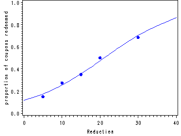
Fig. 14.4, p. 579.
In order to implement logistic regression using proportions it is necessary to use
proc genmod and specify the distribution and the link function. The
parameter estimates in the output correspond to the fitted response function
(14.28) at the bottom of p. 578.

proc genmod data=ch14tab02;
  model r/n = x / dist = bin link = logit lrci;
  output out=temp p=predicted;
run;

The GENMOD Procedure

Model Information

Data Set WORK.CH14TAB02
Distribution Binomial
Link Function Logit
Response Variable (Events) r coupons redeemed
Response Variable (Trials) n no. households
Observations Used 5
Number Of Events 392
Number Of Trials 1000

Criteria For Assessing Goodness Of Fit

Criterion DF Value Value/DF

Deviance 3 2.1668 0.7223
Scaled Deviance 3 2.1668 0.7223
Pearson Chi-Square 3 2.1486 0.7162
Scaled Pearson X2 3 2.1486 0.7162
Log Likelihood -595.9863

Algorithm converged.

Analysis Of Parameter Estimates

Standard Likelihood Ratio 95% Chi-
Parameter DF Estimate Error Confidence Limits Square Pr > ChiSq

Intercept 1 -2.0443 0.1610 -2.3655 -1.7340 161.28 <.0001
x 1 0.0968 0.0085 0.0803 0.1139 128.29 <.0001
Scale 0 1.0000 0.0000 1.0000 1.0000

NOTE: The scale parameter was held fixed.

Fig. 14.4, p. 579. Fitted values for X=0 and X=40 have been added in order for the fitted
curve to extend beyond the range of the X variable in the data set.

data extra;
  if _n_ = 1 then do;
  predicted = exp(-2.04435) / (1+ exp(-2.04435) ); 
  x=0; output;
  predicted = exp(-2.04435 + 0.096834*40) / (1+ exp(-2.04435 + 0.096834*40) ); 
  x=40; output;
  end;
  set temp;
  output;
run;
 
proc sort data = extra;
 by x;
run; 
 
symbol1 v=dot c=blue;
symbol2 i=spline v=none c=blue;
axis1 label=(angle = 90 h = 1) order=(0 to 1.0 by .2);
axis2 order=(0 to 40 by 10); 
proc gplot data = extra;
  plot (p predicted)*x / overlay vaxis=axis1 haxis=axis2;
run;
quit;
goptions reset = all;

Inputting the Disease Outbreak data, table 14.3, p. 583.

data ch14tab03;
  input id x1 socio x4 y x5;
  label  id = 'case'
         x1 = 'age'
      socio = 'socioeconomic status' 
         x4 = 'sector'
          y = 'Disease status'
         x5 = 'savings';
cards;
      1     33      1      1      0      1
      2     35      1      1      0      1
      3      6      1      1      0      0
      4     60      1      1      0      1
      5     18      3      1      1      0
      6     26      3      1      0      0
      7      6      3      1      0      0
      8     31      2      1      1      1
      9     26      2      1      1      0
     10     37      2      1      0      0
     11     23      1      1      0      0
     12     23      1      1      0      0
     13     27      1      1      0      1
     14      9      1      1      1      1
     15     37      1      2      1      1
     16     22      1      2      1      1
     17     67      1      2      1      1
     18      8      1      2      0      1
     19      6      1      2      1      1
     20     15      1      2      1      1
     21     21      2      2      1      1
     22     32      2      2      1      1
     23     16      1      2      1      1
     24     11      2      2      0      0
     25     14      3      2      0      0
     26      9      2      2      0      0
     27     18      2      2      0      0
     28      2      3      1      0      0
     29     61      3      1      0      1
     30     20      3      1      0      0
     31     16      3      1      0      0
     32      9      2      1      0      0
     33     35      2      1      0      1
     34      4      1      1      0      1
     35     44      3      2      0      0
     36     11      3      2      1      0
     37      3      2      2      0      1
     38      6      3      2      0      0
     39     17      2      2      1      0
     40      1      3      2      0      1
     41     53      2      2      1      1
     42     13      1      2      1      0
     43     24      1      2      0      0
     44     70      1      2      1      1
     45     16      3      2      1      1
     46     12      2      2      0      1
     47     20      3      2      1      1
     48     65      3      2      0      1
     49     40      2      2      1      0
     50     38      2      2      1      1
     51     68      2      2      1      1
     52     74      1      2      1      1
     53     14      1      2      1      1
     54     27      1      2      1      1
     55     31      1      2      0      1
     56     18      1      2      0      1
     57     39      1      2      0      0
     58     50      1      2      0      1
     59     31      1      2      0      1
     60     61      1      2      0      1
     61     18      3      1      0      0
     62      5      3      1      0      0
     63      2      3      1      0      1
     64     16      3      1      0      0
     65     59      3      1      1      1
     66     22      3      1      0      0
     67     24      1      1      0      1
     68     30      1      1      0      1
     69     46      1      1      0      1
     70     28      1      1      0      0
     71     27      1      1      0      1
     72     27      1      1      1      0
     73     28      1      1      0      1
     74     52      1      1      1      1
     75     11      3      1      0      1
     76      6      2      1      0      1
     77     46      3      1      0      0
     78     20      2      1      1      1
     79      3      1      1      0      1
     80     18      2      1      0      0
     81     25      2      1      0      0
     82      6      3      1      0      1
     83     65      3      1      1      1
     84     51      3      1      0      1
     85     39      2      1      0      1
     86      8      1      1      0      1
     87      8      2      1      0      0
     88     14      3      1      0      0
     89      6      3      1      0      0
     90      6      3      1      0      1
     91      7      3      1      0      0
     92      4      3      1      0      0
     93      8      3      1      0      0
     94      9      2      1      0      0
     95     32      3      1      1      0
     96     19      3      1      0      0
     97     11      3      1      0      0
     98     35      3      1      0      0
;
run;

Creating the dummy variables for socioeconomic status.

data ch14tb03a;
  set ch14tab03;
  x2 = 0;
  if socio = 2 then x2 = 1;
  x3 = 0;
  if socio = 3 then x3 = 1;
run;

Table 14.4, p. 584. It is the option covb in the model statement that gives
us part b of the table.
Note: The estimate for the intercept is different from the book perhaps because the authors
used a slightly different algorithm. However, it is usually the odds ratio of the other
parameters estimates that are of interest and they are the same as in the book.

proc logistic data = ch14tb03a descending;
  model y = x1 x2 x3 x4/ covb;
run;

The LOGISTIC Procedure

Model Information

Data Set WORK.CH14TB03A
Response Variable y Disease status
Number of Response Levels 2
Number of Observations 98
Link Function Logit
Optimization Technique Fisher’s scoring

Response Profile

Ordered Total
Value y Frequency
1 1 31
2 0 67

Model Convergence Status

Convergence criterion (GCONV=1E-8) satisfied.

Model Fit Statistics

Intercept
Intercept and
Criterion Only Covariates

AIC 124.318 111.054
SC 126.903 123.979
-2 Log L 122.318 101.054

Testing Global Null Hypothesis: BETA=0

Test Chi-Square DF Pr > ChiSq

Likelihood Ratio 21.2635 4 0.0003
Score 20.4067 4 0.0004
Wald 16.6437 4 0.0023

The LOGISTIC Procedure

Analysis of Maximum Likelihood Estimates

Standard
Parameter DF Estimate Error Chi-Square Pr > ChiSq

Intercept 1 -3.8874 0.9955 15.2496 <.0001
x1 1 0.0297 0.0135 4.8535 0.0276
x2 1 0.4088 0.5990 0.4657 0.4950
x3 1 -0.3051 0.6041 0.2551 0.6135
x4 1 1.5746 0.5016 9.8543 0.0017

Odds Ratio Estimates

Point 95% Wald
Effect Estimate Confidence Limits

x1 1.030 1.003 1.058
x2 1.505 0.465 4.868
x3 0.737 0.226 2.408
x4 4.829 1.807 12.907

Association of Predicted Probabilities and Observed Responses

Percent Concordant 77.5 Somers’ D 0.554
Percent Discordant 22.1 Gamma 0.556
Percent Tied 0.3 Tau-a 0.242
Pairs 2077 c 0.777

Estimated Covariance Matrix

Variable Intercept x1 x2 x3 x4

Intercept 0.990945 -0.00605 -0.19645 -0.26324 -0.41483
x1 -0.00605 0.000182 0.00115 0.000732 0.000338
x2 -0.19645 0.00115 0.358793 0.148217 0.012887
x3 -0.26324 0.000732 0.148217 0.364944 0.062267
x4 -0.41483 0.000338 0.012887 0.062267 0.251609

Testing multiple parameters, p. 589.
In SAS testing linear hypotheses about the regression
coefficients is done using a Wald test. To use the built in SAS option just add
test statements for all the hypothesis that needs to be tested. The partial deviance
can be used by running the full and reduced model for each hypothesis and then taking
each model and comparing this difference to the appropriate chi-square distribution.

proc logistic data = ch14tb03a descending;
  model y = x1 x2 x3 x4;
  test: test x1=0;
run;
proc logistic data = ch14tb03a descending;
  model y = x2 x3 x4;
run;

The LOGISTIC Procedure

Model Information

Data Set WORK.CH14TB03A
Response Variable y Disease status
Number of Response Levels 2
Number of Observations 98
Link Function Logit
Optimization Technique Fisher’s scoring

Response Profile

Ordered Total
Value y Frequency

1 1 31
2 0 67

Model Convergence Status

Convergence criterion (GCONV=1E-8) satisfied.

Model Fit Statistics

Intercept
Intercept and
Criterion Only Covariates

AIC 124.318 111.054
SC 126.903 123.979
-2 Log L 122.318 101.054

Testing Global Null Hypothesis: BETA=0

Test Chi-Square DF Pr > ChiSq

Likelihood Ratio 21.2635 4 0.0003
Score 20.4067 4 0.0004
Wald 16.6437 4 0.0023

The LOGISTIC Procedure

Analysis of Maximum Likelihood Estimates

Standard
Parameter DF Estimate Error Chi-Square Pr > ChiSq

Intercept 1 -3.8874 0.9955 15.2496 <.0001
x1 1 0.0297 0.0135 4.8535 0.0276
x2 1 0.4088 0.5990 0.4657 0.4950
x3 1 -0.3051 0.6041 0.2551 0.6135
x4 1 1.5746 0.5016 9.8543 0.0017

Odds Ratio Estimates

Point 95% Wald
Effect Estimate Confidence Limits

x1 1.030 1.003 1.058
x2 1.505 0.465 4.868
x3 0.737 0.226 2.408
x4 4.829 1.807 12.907

Association of Predicted Probabilities and Observed Responses

Percent Concordant 77.5 Somers’ D 0.554
Percent Discordant 22.1 Gamma 0.556
Percent Tied 0.3 Tau-a 0.242
Pairs 2077 c 0.777

Linear Hypotheses Testing Results

Wald
Label Chi-Square DF Pr > ChiSq

test 4.8535 1 0.0276

The LOGISTIC Procedure

Model Information

Data Set WORK.CH14TB03A
Response Variable y Disease status
Number of Response Levels 2
Number of Observations 98
Link Function Logit
Optimization Technique Fisher’s scoring

Response Profile

Ordered Total
Value y Frequency

1 1 31
2 0 67

Model Convergence Status

Convergence criterion (GCONV=1E-8) satisfied.

Model Fit Statistics

Intercept
Intercept and
Criterion Only Covariates

AIC 124.318 114.204
SC 126.903 124.544
-2 Log L 122.318 106.204

Testing Global Null Hypothesis: BETA=0

Test Chi-Square DF Pr > ChiSq

Likelihood Ratio 16.1139 3 0.0011
Score 15.8641 3 0.0012
Wald 14.2743 3 0.0026

The LOGISTIC Procedure

Analysis of Maximum Likelihood Estimates

Standard
Parameter DF Estimate Error Chi-Square Pr > ChiSq

Intercept 1 -3.0595 0.8639 12.5427 0.0004
x2 1 0.2351 0.5752 0.1670 0.6828
x3 1 -0.4779 0.5829 0.6721 0.4123
x4 1 1.6203 0.4857 11.1289 0.0008

Odds Ratio Estimates

Point 95% Wald
Effect Estimate Confidence Limits

x2 1.265 0.410 3.906
x3 0.620 0.198 1.944
x4 5.055 1.951 13.095

Association of Predicted Probabilities and Observed Responses

Percent Concordant 65.8 Somers’ D 0.465
Percent Discordant 19.3 Gamma 0.546
Percent Tied 14.9 Tau-a 0.203
Pairs 2077 c 0.733

Creating all the interactions to be tested.

data ch14tb03b;
  set ch14tb03a;
  x1x2 = x1*x2;
  x1x3 = x1*x3;
  x1x4 = x1*x4;
  x2x4 = x2*x4;
  x3x4 = x3*x4;
run;

Testing the interactions, p. 589.

proc logistic data = ch14tb03b descending;
  model y = x1-x4 x1x2 x1x3 x1x4 x2x4 x3x4;
  test: test x1x2=x1x3= x1x4= x2x4= x3x4=0;
run;

The LOGISTIC Procedure

Model Information

Data Set WORK.CH14TB03B
Response Variable y Disease status
Number of Response Levels 2
Number of Observations 98
Link Function Logit
Optimization Technique Fisher’s scoring

Response Profile

Ordered Total
Value y Frequency

1 1 31
2 0 67

Model Convergence Status
Convergence criterion (GCONV=1E-8) satisfied.

Model Fit Statistics

Intercept
Intercept and
Criterion Only Covariates

AIC 124.318 113.996
SC 126.903 139.846
-2 Log L 122.318 93.996

Testing Global Null Hypothesis: BETA=0

Test Chi-Square DF Pr > ChiSq

Likelihood Ratio 28.3217 9 0.0008
Score 25.6302 9 0.0023
Wald 17.9067 9 0.0363

The LOGISTIC Procedure

Analysis of Maximum Likelihood Estimates

Standard
Parameter DF Estimate Error Chi-Square Pr > ChiSq

Intercept 1 -5.5161 2.2471 6.0260 0.0141
x1 1 0.0646 0.0583 1.2294 0.2675
x2 1 -1.7862 3.0841 0.3354 0.5625
x3 1 0.2955 2.2550 0.0172 0.8957
x4 1 2.9796 1.2481 5.6988 0.0170
x1x2 1 0.1054 0.0559 3.5514 0.0595
x1x3 1 0.0140 0.0316 0.1952 0.6586
x1x4 1 -0.0342 0.0309 1.2231 0.2688
x2x4 1 -0.3094 1.4409 0.0461 0.8300
x3x4 1 -0.7396 1.2489 0.3507 0.5537

Odds Ratio Estimates

Point 95% Wald
Effect Estimate Confidence Limits

x1 1.067 0.952 1.196
x2 0.168 <0.001 70.702
x3 1.344 0.016 111.632
x4 19.680 1.705 227.221
x1x2 1.111 0.996 1.240
x1x3 1.014 0.953 1.079
x1x4 0.966 0.910 1.027
x2x4 0.734 0.044 12.363
x3x4 0.477 0.041 5.519

Association of Predicted Probabilities and Observed Responses

Percent Concordant 80.4 Somers’ D 0.610
Percent Discordant 19.4 Gamma 0.612
Percent Tied 0.3 Tau-a 0.267
Pairs 2077 c 0.805

Linear Hypotheses Testing Results

Wald
Label Chi-Square DF Pr > ChiSq

test 5.9413 5 0.3120

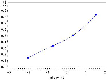
Example 1, p. 591 and Fig. 14.5, p. 592.
Invoking the macro diag_plot.
Note: The macro splits the observations into groups with an equal number of observations
except for the last group therefore they may not match the groups in the book since
they are not the same size as those in the book. Also, the results from the
logistic regression produced by the macro has been
omitted.

%include "c:neter/sas/examples/alsm/diag_plot.sas";
%diag_plot(ch14tab01, y, x, 4);

Obs    class       min         max      midpoint    n       pj
 1       1      -2.41375    -1.60632    -2.01004    7    0.14286

 2       2      -1.28335    -0.15295    -0.71815    6    0.33333

 3       3      -0.15295     0.81597     0.33151    6    0.50000

 4       4       0.97745     2.10785     1.54265    6    0.83333

Example 2, p. 591 and Fig. 14.6, p. 592.
Invoking the macro diag_plot again and again the results from the logistic
regression produced by the macro has been omitted.


 %diag_plot(ch14tb03a, y, x1 x2 x3 x4, 5);

Obs    class       min         max      midpoint     n       pj
 1       1      -2.55835    -2.08241    -2.32038    20    0.05000

 2       2      -2.07476    -1.47983    -1.77729    20    0.15000

 3       3      -1.42033    -0.74386    -1.08210    19    0.26316

 4       4      -0.71601     0.06505    -0.32548    20    0.55000

 5       5       0.17633     1.69341     0.93487    19    0.57895

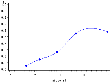
Table 14.5, p. 594.
Note: The numbers are not exactly the same as those in the book most probably due to rounding
errors. Only the output from the final print procedure has been included in the results.

proc logistic data = ch14tb03a descending;
  model y = x1 x2 x3 x4 ;
  output out=temp p = pi;
run;
data temp;
  set temp;
  pihat = log( pi / (1 - pi) );
run;
proc sort data = temp;
  by pihat;
run;
data temp;
  set temp nobs=total;
  class = .;
  class = int( ( _n_ - 1 )/( total/5 ) ) +1;
run;
proc sql;
  create table temp1 as
  select *, max(pihat) as max, min(pihat) as min, sum(pi) as Ej1, count(pi) as n,
            sum(y) as Oj1, count(pi) - sum(pi) as Ej0, count(pi) - sum(y) as Oj0
  from temp
  group by class;
quit;
proc sort data = temp1 (keep = class n min max  Oj0 Ej0 Oj1 Ej1);
  by class ;
run;
data temp1;
  set temp1;
  by class;
  if first.class;
run;
proc print data=temp1;
  var class min max n Oj0 Ej0 Oj1 Ej1;
run;

Obs    class       min         max       n    Oj0      Ej0      Oj1      Ej1
 1       1      -2.55835    -2.08241    20     19    18.1952      1     1.8048

 2       2      -2.07476    -1.47983    20     17    16.9072      3     3.0928

 3       3      -1.42033    -0.74386    19     14    14.0400      5     4.9600

 4       4      -0.71601     0.06505    20      9    11.5587     11     8.4413

 5       5       0.17633     1.69341    19      8     6.2976     11    12.7024

Index plots, including the RESDEV (Residual deviance) plot which is the same as
Fig. 14.7, p. 596.

proc logistic data = ch14tab01 desc;
  model y = x / iplots;
run;

The LOGISTIC Procedure

Model Information

Data Set WORK.CH14TAB01
Response Variable y Success
Number of Response Levels 2
Number of Observations 25
Link Function Logit
Optimization Technique Fisher’s scoring

Response Profile

Ordered Total
Value y Frequency

1 1 11
2 0 14

Model Convergence Status

Convergence criterion (GCONV=1E-8) satisfied.

Model Fit Statistics

Intercept
Intercept and
Criterion Only Covariates

AIC 36.296 29.425
SC 37.515 31.862
-2 Log L 34.296 25.425

Testing Global Null Hypothesis: BETA=0

Test Chi-Square DF Pr > ChiSq

Likelihood Ratio 8.8719 1 0.0029
Score 7.9742 1 0.0047
Wald 6.1760 1 0.0129

Analysis of Maximum Likelihood Estimates

Standard
Parameter DF Estimate Error Chi-Square Pr > ChiSq

Intercept 1 -3.0597 1.2594 5.9029 0.0151
x 1 0.1615 0.0650 6.1760 0.0129

The LOGISTIC Procedure

Odds Ratio Estimates

Point 95% Wald
Effect Estimate Confidence Limits

x 1.175 1.035 1.335

Association of Predicted Probabilities and Observed Responses

Percent Concordant 82.5 Somers’ D 0.662
Percent Discordant 16.2 Gamma 0.671
Percent Tied 1.3 Tau-a 0.340
Pairs 154 c 0.831

The LOGISTIC Procedure

—–+————–+————–+————–+————–+————–+——
RESCHI | |
P 4 + +
e | |
a | |
r | * |
s 2 + +
o | * |
n | * * * * |
| * * * * * |
R 0 + +
e | * * * * * * * * * * |
s | * * |
i | * |
d -2 + +
u | * |
a | |
l | |
-4 + +
| |
—–+————–+————–+————–+————–+————–+——
0 5 10 15 20 25

Case Number INDEX

—–+————–+————–+————–+————–+————–+——
2 + * +
D | |
e | * |
v | * |
i RESDEV | * |
a | * * * |
n | * * * |
c | * |
e | |
0 + +
R | |
e | * * * * * |
s | * * * |
i | * * |
d | * * |
u | |
a | * |
l | |
-2 + * +
—–+————–+————–+————–+————–+————–+——
0 5 10 15 20 25

Case Number INDEX

The LOGISTIC Procedure

——+————–+————–+————–+————–+————–+——-
0.12 + +
| |
| |
H | |
a | * * * |
t | * * |
0.10 + +
D | |
i | |
a H | * |
g | |
o | * |
n 0.08 + * * * * * * * +
a | |
l | * * * |
| * |
| * * |
| * * |
0.06 + * * * +
——+————–+————–+————–+————–+————–+——-
0 5 10 15 20 25

Case Number INDEX

—–+————–+————–+————–+————–+————–+—–
1.0 + +
I | |
n | |
t | * |
e | |
r | |
c 0.5 + +
e | * |
p | * |
t DFBETA0 | |
| * |
D | * |
f 0.0 + * * * +
B | * * * * * * * * * * * * |
e | * * * * * |
t | |
a | |
| |
-0.5 + +
—–+————–+————–+————–+————–+————–+—–
0 5 10 15 20 25

Case Number INDEX

The LOGISTIC Procedure

—–+————–+————–+————–+————–+————–+—–
0.5 + +
| |
| |
| |
| * * * * |
x | * * * * * * * * * * * * * * |
0.0 + * * * +
D | |
f | |
B DFBETA1 | * |
e | * |
t | |
a -0.5 + +
| * |
| * |
| |
| |
| |
-1.0 + +
—–+————–+————–+————–+————–+————–+—–
0 5 10 15 20 25

Case Number INDEX

——+————–+————–+————–+————–+————–+——-
C 0.75 + +
o | |
n | * |
f | |
i | |
d | * |
e 0.50 + +
n | |
c | |
e C | |
| |
I | |
n 0.25 + +
t | * * |
e | |
r | |
v | * * |
a | * * * * * * * * * * * * |
l 0.00 + * * * * * * * +
——+————–+————–+————–+————–+————–+——-
D 0 5 10 15 20 25
i
Case Number INDEX

The LOGISTIC Procedure

——+————–+————–+————–+————–+————–+——-
C 0.6 + * +
o | |
n | |
f | * |
i | |
d | |
e 0.4 + +
n | |
c | |
e CBAR | |
| |
I | |
n 0.2 + * * +
t | |
e | |
r | |
v | * * * * |
a | * * * * * * * * * * * |
l 0.0 + * * * * * * +
——+————–+————–+————–+————–+————–+——-
D 0 5 10 15 20 25
i
Case Number INDEX

—–+————–+————–+————–+————–+————–+——
6 + +
| |
D | |
e | |
l | |
t | * * |
a 4 + +
| |
D | |
e DIFDEV | |
v | * * |
i | |
a 2 + +
n | * |
c | * * * |
e | * * |
| * * * * * |
| * * * * * * * * * * |
0 + +
—–+————–+————–+————–+————–+————–+——
0 5 10 15 20 25

Case Number INDEX

The LOGISTIC Procedure

—-+————–+————–+————–+————–+————–+—–
DIFCHISQ | |
8 + +
D | |
e | |
l | * |
t 6 + +
a | * |
| |
C | |
h 4 + +
i | |
S | * |
q | * |
u 2 + +
a | |
r | * * * * |
e | * * * * * * * * |
0 + * * * * * * * * * +
| |
—-+————–+————–+————–+————–+————–+—–
0 5 10 15 20 25

Case Number INDEX

Predicting mean responses with confidence interval, example p. 604-605.
The output contains the point estimate of the logit mean response as phat,
the confidence limits for the logit mean response as lower1 and upper1, the point
estimate for the mean response as p, and finally, the confidence interval for the mean
response as lower and upper. The output from the proc logistic is not shown.

data ch14tb03b;
  if _n_ = 1 then do;
    id = 99; x1=10; x2=0; x3=1; x4=1;
    end;
  output;
  set ch14tb03a;
run;
proc logistic data = ch14tb03b desc;
  model y = x1 x2 x3 x4;
  output out=temp p=p upper=upper lower=lower;
run;
data temp;
  set temp;
  lower1 = log(lower/ (1-lower) ) ;
  upper1 = log(upper / (1-upper) );
  phat = log(p / (1-p) );
run;
proc print data = temp;
  where id = 99;
  var  phat lower1 upper1 p lower upper;
run;

Obs phat lower1 upper1 p lower upper

1 -2.32038 -3.38397 -1.25679 0.089449 0.032800 0.22153

Table 14.7, p. 607.
The table produced by SAS is very different from the table in the book. The book uses the list of predicted fitted values and then compares them to a specified cutoff point. SAS
does not use this method because when you classify binary data and the observations that are
used to fit the model are also used to estimate the classification error then the resulting
error-count estimate is biased. One way to reduce the bias is to remove the observation to be
classified and re-estimate the parameters of the model and then classify the observation
based on the parameter estimates based on the smaller dataset (without the observation to be
classified). In order to increase efficiency SAS uses a one-step approximation of the
parameter estimates based on the smaller dataset (without the observation to be classified).
For the details of the one-step approximation please refer to the manual under Proc Logistic
Classification Table.

proc logistic data = ch14tb03a desc;
  model y = x1 x2 x3 x4/ ctable;
  output out=temp p=p;
run;

The LOGISTIC Procedure

Model Information

Data Set WORK.CH14TB03A
Response Variable y Disease status
Number of Response Levels 2
Number of Observations 98
Link Function Logit
Optimization Technique Fisher’s scoring

Response Profile

Ordered Total
Value y Frequency

1 1 31
2 0 67

Model Convergence Status

Convergence criterion (GCONV=1E-8) satisfied.

Model Fit Statistics

Intercept
Intercept and
Criterion Only Covariates

AIC 124.318 111.054
SC 126.903 123.979
-2 Log L 122.318 101.054

Testing Global Null Hypothesis: BETA=0

Test Chi-Square DF Pr > ChiSq

Likelihood Ratio 21.2635 4 0.0003
Score 20.4067 4 0.0004
Wald 16.6437 4 0.0023

The LOGISTIC Procedure

Analysis of Maximum Likelihood Estimates

Standard
Parameter DF Estimate Error Chi-Square Pr > ChiSq

Intercept 1 -3.8874 0.9955 15.2496 <.0001
x1 1 0.0297 0.0135 4.8535 0.0276
x2 1 0.4088 0.5990 0.4657 0.4950
x3 1 -0.3051 0.6041 0.2551 0.6135
x4 1 1.5746 0.5016 9.8543 0.0017

Odds Ratio Estimates

Point 95% Wald
Effect Estimate Confidence Limits

x1 1.030 1.003 1.058
x2 1.505 0.465 4.868
x3 0.737 0.226 2.408
x4 4.829 1.807 12.907

Association of Predicted Probabilities and Observed Responses

Percent Concordant 77.5 Somers’ D 0.554
Percent Discordant 22.1 Gamma 0.556
Percent Tied 0.3 Tau-a 0.242
Pairs 2077 c 0.777

Classification Table

Correct Incorrect Percentages
Prob Non- Non- Sensi- Speci- False False
Level Event Event Event Event Correct tivity ficity POS NEG

0.060 31 0 67 0 31.6 100.0 0.0 68.4 .
0.080 31 4 63 0 35.7 100.0 6.0 67.0 0.0
0.100 29 12 55 2 41.8 93.5 17.9 65.5 14.3
0.120 29 22 45 2 52.0 93.5 32.8 60.8 8.3
0.140 28 23 44 3 52.0 90.3 34.3 61.1 11.5
0.160 27 25 42 4 53.1 87.1 37.3 60.9 13.8
0.180 26 32 35 5 59.2 83.9 47.8 57.4 13.5
0.200 26 36 31 5 63.3 83.9 53.7 54.4 12.2
0.220 25 39 28 6 65.3 80.6 58.2 52.8 13.3
0.240 23 41 26 8 65.3 74.2 61.2 53.1 16.3
0.260 22 42 25 9 65.3 71.0 62.7 53.2 17.6
0.280 20 43 24 11 64.3 64.5 64.2 54.5 20.4
0.300 20 45 22 11 66.3 64.5 67.2 52.4 19.6
0.320 19 46 21 12 66.3 61.3 68.7 52.5 20.7
0.340 18 48 19 13 67.3 58.1 71.6 51.4 21.3

The LOGISTIC Procedure

Classification Table

Correct Incorrect Percentages
Prob Non- Non- Sensi- Speci- False False
Level Event Event Event Event Correct tivity ficity POS NEG

0.360 17 50 17 14 68.4 54.8 74.6 50.0 21.9
0.380 16 51 16 15 68.4 51.6 76.1 50.0 22.7
0.400 14 51 16 17 66.3 45.2 76.1 53.3 25.0
0.420 13 53 14 18 67.3 41.9 79.1 51.9 25.4
0.440 13 53 14 18 67.3 41.9 79.1 51.9 25.4
0.460 12 53 14 19 66.3 38.7 79.1 53.8 26.4
0.480 12 55 12 19 68.4 38.7 82.1 50.0 25.7
0.500 11 55 12 20 67.3 35.5 82.1 52.2 26.7
0.520 10 56 11 21 67.3 32.3 83.6 52.4 27.3
0.540 10 58 9 21 69.4 32.3 86.6 47.4 26.6
0.560 9 59 8 22 69.4 29.0 88.1 47.1 27.2
0.580 8 61 6 23 70.4 25.8 91.0 42.9 27.4
0.600 8 62 5 23 71.4 25.8 92.5 38.5 27.1
0.620 8 62 5 23 71.4 25.8 92.5 38.5 27.1
0.640 7 64 3 24 72.4 22.6 95.5 30.0 27.3
0.660 7 64 3 24 72.4 22.6 95.5 30.0 27.3
0.680 6 64 3 25 71.4 19.4 95.5 33.3 28.1
0.700 5 64 3 26 70.4 16.1 95.5 37.5 28.9
0.720 5 65 2 26 71.4 16.1 97.0 28.6 28.6
0.740 5 65 2 26 71.4 16.1 97.0 28.6 28.6
0.760 3 65 2 28 69.4 9.7 97.0 40.0 30.1
0.780 2 65 2 29 68.4 6.5 97.0 50.0 30.9
0.800 1 67 0 30 69.4 3.2 100.0 0.0 30.9
0.820 1 67 0 30 69.4 3.2 100.0 0.0 30.9
0.840 0 67 0 31 68.4 0.0 100.0 . 31.6

Inputting the validation data set which is the remaining data from Data Set C.3, p. 1370.

data validation;
  input id x1 socio x4 y x5;
  label  id = 'case'
         x1 = 'age'
      socio = 'socioeconomic status' 
         x4 = 'sector'
          y = 'Disease status'
         x5 = 'savings';
cards;
     99     16      1      1      0      0
    100      1      1      1      0      1
    101      6      1      1      0      1
    102     27      1      1      0      1
    103     25      1      1      0      1
    104     18      1      1      0      0
    105     37      3      1      0      0
    106     33      3      1      1      0
    107     27      2      1      0      0
    108      2      1      1      0      0
    109      8      2      1      0      0
    110      5      1      1      0      0
    111      1      1      1      0      1
    112     32      1      1      0      0
    113     25      1      1      1      1
    114     15      1      2      0      0
    115     15      1      2      0      1
    116     26      1      2      0      1
    117     42      1      2      1      1
    118      7      1      2      0      1
    119      2      1      2      0      0
    120     65      1      2      1      1
    121     33      2      2      0      1
    122      8      2      2      1      0
    123     30      2      2      0      0
    124      5      3      2      0      0
    125     15      3      2      0      0
    126     60      3      2      1      1
    127     13      3      2      1      1
    128     70      3      1      0      1
    129      5      3      1      0      0
    130      3      3      1      0      1
    131     50      2      1      0      1
    132      6      2      1      0      0
    133     12      2      1      0      1
    134     39      3      2      1      0
    135     15      2      2      0      1
    136     35      2      2      1      0
    137      2      2      2      0      1
    138     17      3      2      0      0
    139     43      3      2      1      1
    140     30      2      2      0      1
    141     11      1      2      0      1
    142     39      1      2      1      1
    143     32      1      2      0      1
    144     17      1      2      0      1
    145      3      3      2      0      1
    146      7      3      2      0      0
    147      2      2      2      0      0
    148     64      2      2      1      1
    149     13      1      2      1      2
    150     15      2      2      1      1
    151     48      2      2      0      1
    152     23      1      2      0      1
    153     48      1      2      1      0
    154     25      1      2      0      1
    155     12      1      2      0      1
    156     46      1      2      1      1
    157     79      1      2      0      1
    158     56      1      2      0      1
    159      8      1      2      0      1
    160     29      3      1      1      0
    161     35      3      1      1      0
    162     11      3      1      1      0
    163     69      3      1      0      1
    164     21      3      1      1      0
    165     13      3      1      0      0
    166     21      1      1      0      1
    167     32      1      1      1      1
    168     24      1      1      1      0
    169     24      1      1      0      1
    170     73      1      1      0      1
    171     42      1      1      0      1
    172     34      1      1      1      1
    173     30      2      1      0      0
    174      7      2      1      0      0
    175     29      3      1      1      0
    176     22      3      1      1      0
    177     38      2      1      0      1
    178     13      2      1      0      1
    179     12      2      1      0      1
    180     42      3      1      0      0
    181     17      3      1      1      0
    182     21      3      1      0      1
    183     34      1      1      0      1
    184      1      3      1      0      0
    185     14      2      1      0      0
    186     16      2      1      0      0
    187      9      3      1      0      0
    188     53      3      1      0      0
    189     27      3      1      0      0
    190     15      3      1      0      0
    191      9      3      1      0      0
    192      4      2      1      0      1
    193     10      3      1      0      1
    194     31      3      1      0      0
    195     85      3      1      0      1
    196     24      2      1      0      0
;
run;

Creating the dummy variables for the socioeconomic variable.

data validation;
  set validation;
  x2 = 0;
  if socio = 2 then x2 = 1;
  x3 = 0;
  if socio = 3 then x3 = 1;
run;

Creating the fitted values of the validation dataset using parameter estimates from the
Disease Outbreak dataset (table 14.3), p. 608. In order to get the same classification table it was necessary to use 0.7 as the cutoff
value. The percentages shown in the table in the book are the column percentages which are
in the second row of each cell.
Note: The proc format is simply to create nice labels for our table.

data validation1;
  set validation;
  e =  2.3129 - 0.0297*x1 - .4088*x2 + 0.3051*x3 - 1.5746*x4;
  ex = exp(e);
  p = 1/( 1+ ex);
  yes = 0;
  if p >= .7 then yes = 1;
run;
proc format;
  value y 1='with disease' 0='without disease';
  value yes 1='pihat >= .7' 0='piehat < .7';
run;
proc freq data = validation1;
  format y y. yes yes.;
  table yes*y / missing norow nopercent;
run;

The FREQ Procedure
Table of yes by y
yes          y(Disease status)
Frequency   |

Col Pct     |without |with dis|  Total

            |disease |ease    |

————+——–+——–+

piehat < .7 |     44 |     12 |     56

            |  61.11 |  46.15 |

————+——–+——–+

pihat >= .7 |     28 |     14 |     42

            |  38.89 |  53.85 |

————+——–+——–+

Total             72       26       98

Inputting the Miller Lumber Company Example, p. 613.

data ch14tab08;
  input y x1 x2 x3 x4 x5;
  label x1 = 'Housing'
        x2 = 'Income'
		x3 = 'Age'
		x4 = 'Competitor Distance'
		x5 = 'Store Distance'
		 y = 'Costumers';
cards;
 9   606   41393   3  3.04  6.32
 6   641   23635  18  1.95  8.89
28   505   55475  27  6.54  2.05
11   866   64646  31  1.67  5.81
 4   599   31972   7  0.72  8.11
 4   520   41755  23  2.24  6.81
 0   354   46014  26  0.77  9.27
14   483   34626   1  3.51  7.92
16  1034   85207  13  4.23  4.40
13   456   33021  32  3.07  6.03
 9    19   39198  22  2.96  6.09
14   530   38794   5  2.77  6.08
 5   337   30855   1  1.33  9.86
 9   586   28852   7  2.98  8.64
 9  1113  120065   9  3.58  5.26
 7   525   32229   3  1.27  7.56
 4   377   36828  15  1.92  8.91
26  1127   90302  26  5.83  1.74
32   877   51707  27  5.19  3.66
26  1007   89860  55  5.03  2.03
11   657   60513  32  4.38  8.30
12   302   42191  54  3.41  5.21
 3   603   28736  41  0.34  8.29
15   556   49129  33  4.78  3.89
12   635   29308  42  2.53  6.17
 9   386   26734  14  4.99  9.70
14  1011   57862  54  4.60  3.94
10   925   70030  36  4.58  8.66
22   898   46027  44  3.03  5.60
 8   731   32202  43  5.15  9.67
 3   584   32871  13  1.47  8.02
11   439   29564  18  3.67  5.10
 2   153   46806  21  0.84  9.18
 6  1069   59805  22  2.50  9.43
11   443   42555  53  2.62  5.75
10   392   36998   7  1.03  7.74
 0   828   85664   4  1.30  9.66
15   159   21238   4  2.98  8.66
 9   830   47972  40  2.28  9.26
16   234   33246  26  3.95  4.61
29  1004   45927  24  4.90  2.69
 6   643   58315   8  0.78  6.26
26   741   69177   9  6.61  0.87
13   306   40886  27  4.53  2.68
 0   180   44588  14  0.88  9.38
 8   644   47347  35  2.94  7.69
 8   109   31791   9  4.37  9.31
21   809   42740  17  4.10  4.75
12   722   59175  35  2.38  5.09
26  1006   48862  48  5.04  2.21
 3   786   54678  20  3.59  8.52
 7  1041   59835  40  1.68  7.59
 5   524   51756  39  0.57  9.10
 9   725   34817  18  1.88  7.96
13   482   29942  14  3.17  6.91
28   666   68684  25  5.78  2.55
10   450   64790   3  4.35  6.03
12   667   58535  25  2.78  5.59
 6   921   42919  13  2.48  7.69
11   412   40722  32  2.47  9.43
12   526   42120  30  4.29  6.15
11   523   28647  43  2.69  7.54
 9  1066   61464  40  1.15  8.25
 8  1001   70136  29  2.58  9.67
 9   669   34595  38  4.06  8.78
 8   582   30878  58  1.91  6.86
 6   872   39366  52  0.73  8.67
 6   758   61563  31  3.08  8.33
15   782   38412  26  2.72  6.71
15   551   41045   2  3.62  7.45
12   201   23864  43  4.80  8.74
10   730   38647   9  0.67  7.92
 8   738   58387  13  2.01  6.60
 3   469   37242  40  1.42  8.37
10   898   38337  32  2.63  9.56
10   780   68201   5  4.12  6.69
15   622   41066  46  4.48  4.10
 6   391   40873  19  1.67  6.90
 9   531   54655  40  2.32  5.69
21   566   49826   1  3.06  4.03
13   410   29013  50  2.68  7.58
 8   719   78082  31  2.70  4.89
 6   684   57506  51  2.13  8.31
 8   865   47118  46  2.17  9.06
21  1031   72373  48  6.27  1.75
 7   862   67787   1  2.10  8.63
19   758   40305  15  3.95  5.58
13  1141   50026  45  2.79  6.18
24  1289   98701   8  5.87  2.73
 7   674   58195  54  4.30  6.40
 3   683   47991  57  1.54  9.52
 8   650   63123  15  3.17  9.46
 9   406   39051  29  3.11  9.62
18   966  114633  38  6.33  2.22
12  1103   55773  44  4.58  8.68
 8   312   43393  41  2.25  6.43
16   787   61765  53  5.39  3.37
 5   416   33348  48  1.48  7.66
 8   528   44541  31  4.91  9.67
11   919   40795   8  2.97  7.79
12   482   55972   9  2.91  5.85
14   781   33140  30  1.42  5.71
17   120   19673  21  2.65  6.25
17   693   36190   6  4.70  9.54
 6   348   25768  42  1.43  7.11
15   780   53974  47  4.21  6.41
10   752   71814   1  3.13  5.47
 6   817   54429  47  1.90  9.90
 4   268   34022  54  1.20  9.51
 6   519   52850  43  2.92  8.62
;
run;

Table 14.9, p. 613.
Note: In SAS the estimate for beta2 -0.00001169 is rounded to -0.0000.

proc genmod data=ch14tab08;
  model y = x1-x5 / dist = poisson link   = log;
  output out=temp p=muhati resdev=devi;
run;

The GENMOD Procedure

Model Information

Data Set WORK.CH14TAB08
Distribution Poisson
Link Function Log
Dependent Variable y Costumers
Observations Used 110

Criteria For Assessing Goodness Of Fit

Criterion DF Value Value/DF

Deviance 104 114.9854 1.1056
Scaled Deviance 104 114.9854 1.1056
Pearson Chi-Square 104 101.8808 0.9796
Scaled Pearson X2 104 101.8808 0.9796
Log Likelihood 1898.0224

Algorithm converged.

Analysis Of Parameter Estimates

Standard Wald 95% Confidence Chi-
Parameter DF Estimate Error Limits Square Pr > ChiSq

Intercept 1 2.9424 0.2072 2.5362 3.3486 201.57 <.0001
x1 1 0.0006 0.0001 0.0003 0.0009 18.17 <.0001
x2 1 -0.0000 0.0000 -0.0000 -0.0000 30.63 <.0001
x3 1 -0.0037 0.0018 -0.0072 -0.0002 4.37 0.0365
x4 1 0.1684 0.0258 0.1179 0.2189 42.70 <.0001
x5 1 -0.1288 0.0162 -0.1605 -0.0970 63.17 <.0001
Scale 0 1.0000 0.0000 1.0000 1.0000

NOTE: The scale parameter was held fixed.

Table 14.10, p. 614.

proc print data = temp (obs=10);
  var y muhati devi;
run;

Obs y muhati devi

1 9 12.3378 -0.99880
2 6 8.7671 -0.99158
3 28 28.1259 -0.02375
4 11 8.4071 0.85335
5 4 7.2606 -1.32357
6 4 8.8818 -1.83900
7 0 4.2982 -2.93195
8 14 10.9989 0.86785
9 16 14.4440 0.40238
10 13 11.6344 0.39289

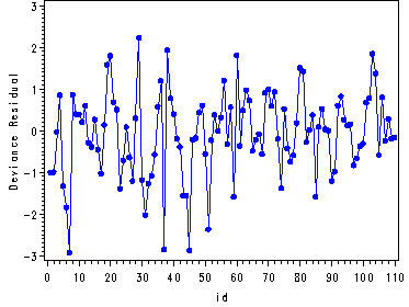
Fig. 14.9, p. 614.
Note: It is necessary to first create an index variable and graph the devi versus the index.

data temp;
  set temp;
  id = _n_;
run;
 
symbol1 v=dot i=join c=blue h = .8;
axis1 label=(angle = 90);
 
proc gplot data = temp;
  plot devi*id/ vaxis = axis1;
run;
quit;