Applied Linear Statistical Models by Neter, Kutner, et. al. Chapter 18: ANOVA Diagnostics and Remedial Measures

Inputting the Rust Inhibitor data, table 17.2a, p. 712.

data Rust;
  input performance brand experiment;
cards;
  43.9  1   1
  39.0  1   2
  46.7  1   3
  43.8  1   4
  44.2  1   5
  47.7  1   6
  43.6  1   7
  38.9  1   8
  43.6  1   9
  40.0  1  10
  89.8  2   1
  87.1  2   2
  92.7  2   3
  90.6  2   4
  87.7  2   5
  92.4  2   6
  86.1  2   7
  88.1  2   8
  90.8  2   9
  89.1  2  10
  68.4  3   1
  69.3  3   2
  68.5  3   3
  66.4  3   4
  70.0  3   5
  68.1  3   6
  70.6  3   7
  65.2  3   8
  63.8  3   9
  69.2  3  10
  36.2  4   1
  45.2  4   2
  40.7  4   3
  40.5  4   4
  39.3  4   5
  40.3  4   6
  43.2  4   7
  38.7  4   8
  40.9  4   9
  39.7  4  10
;
run;

Table 18.1, p. 758.

proc glm data=rust noprint;
  class brand;
  model performance = brand;
  output out=temp r=resid p=predict;
run;
proc freq data=temp;
  weight resid;
  table experiment*brand/ norow nocol nopercent ;
run;

The FREQ Procedure
Table of experiment by brand

experiment     brand
Frequency|       1|       2|       3|       4|  Total

———+——–+——–+——–+——–+

       1 |   0.76 |   0.36 |   0.45 |  -4.27 |   -2.7

———+——–+——–+——–+——–+

       2 |  -4.14 |  -2.34 |   1.35 |   4.73 |   -0.4

———+——–+——–+——–+——–+

       3 |   3.56 |   3.26 |   0.55 |   0.23 |    7.6

———+——–+——–+——–+——–+

       4 |   0.66 |   1.16 |  -1.55 |   0.03 |    0.3

———+——–+——–+——–+——–+

       5 |   1.06 |  -1.74 |   2.05 |  -1.17 |    0.2

———+——–+——–+——–+——–+

       6 |   4.56 |   2.96 |   0.15 |  -0.17 |    7.5

———+——–+——–+——–+——–+

       7 |   0.46 |  -3.34 |   2.65 |   2.73 |    2.5

———+——–+——–+——–+——–+

       8 |  -4.24 |  -1.34 |  -2.75 |  -1.77 |  -10.1

———+——–+——–+——–+——–+

       9 |   0.46 |   1.36 |  -4.15 |   0.43 |   -1.9

———+——–+——–+——–+——–+

      10 |  -3.14 |  -0.34 |   1.25 |  -0.77 |     -3

———+——–+——–+——–+——–+

Total           0        0  -28E-15  377E-15  348E-15

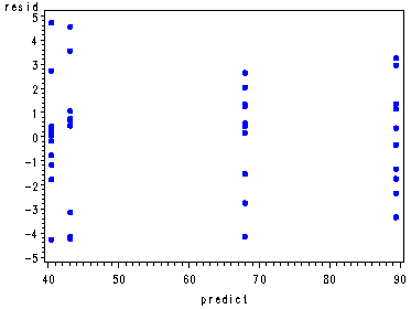
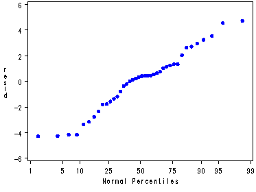
Univariate analysis of the residual, fig. 18.1, p. 759.

goptions reset=all;
symbol v=dot c=blue h=.8;
proc gplot data=temp;
  plot resid*predict;
run;
quit;
proc univariate data=temp noprint;
  var resid;
  probplot resid;
run;

Inputting ABT Electronics data, table 18.2, p. 765.

data Electronics;
  input strength type joint;
cards;
  14.87  1  1
  16.81  1  2
  15.83  1  3
  15.47  1  4
  13.60  1  5
  14.76  1  6
  17.40  1  7
  14.62  1  8
  18.43  2  1
  18.76  2  2
  20.12  2  3
  19.11  2  4
  19.81  2  5
  18.43  2  6
  17.16  2  7
  16.40  2  8
  16.95  3  1
  12.28  3  2
  12.00  3  3
  13.18  3  4
  14.99  3  5
  15.76  3  6
  19.35  3  7
  15.52  3  8
   8.59  4  1
  10.90  4  2
   8.60  4  3
  10.13  4  4
  10.28  4  5
   9.98  4  6
   9.41  4  7
  10.04  4  8
  11.55  5  1
  13.36  5  2
  13.64  5  3
  12.16  5  4
  11.62  5  5
  12.39  5  6
  12.05  5  7
  11.95  5  8
;
run;

Table 18.2, the mean, median and variance of pull strength by flux type, p. 765.

proc means data=electronics mean median var;
  class type;
  var strength;
run;

The MEANS Procedure

Analysis Variable : strength

N
type Obs Mean Median Variance
——————————————————————-
1 8 15.4200000 15.1700000 1.5305143
2 8 18.5275000 18.5950000 1.5699357
3 8 15.0037500 15.2550000 6.1833982
4 8 9.7412500 10.0100000 0.6668411
5 8 12.3400000 12.1050000 0.5920000
——————————————————————-

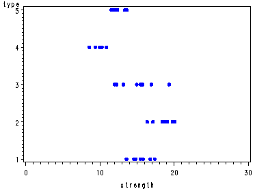
Fig. 18.6, p. 766.

goptions reset=all;
symbol v=dot c=blue h=.8;
axis1 order=(0 to 30 by 10);
proc gplot data=electronics;
  plot type*strength / haxis=axis1;
run;
quit;

The Hartley test for equal variances.
Note: SAS does not have the an inverse Hartley distribution function, so the critical value has
to be obtained from another source.

ods listing close;
proc means data=electronics var;
  class type;
  var strength;
  ods output summary=temp;
run;
ods listing;
ods output close;
proc sql;
  select max(Strength_Var) as max, min(Strength_Var) as min,  9.70 as critvalue,
         max(Strength_Var)/min(Strength_Var) as H 
  from temp;
quit;

     max       min  critvalue         H

—————————————

6.183398     0.592     9.7000  10.44493

Modified Levene Test, p. 767.

proc reg data=electronics noprint;
  model strength = type;
  output out=temp r=r;
run;
proc means data = temp noprint;
  by type;
  var r;
  output out=mout median=mr;
run;
proc print data = mout;
 var type mr;
run;
data mtemp;
  merge temp mout;
  by type;
  d = abs(r - mr);
run; 
proc anova data=mtemp;
  class type;
  model d = type;
run;
quit;

Obs type mr

1 1 -2.02575
2 2 2.89387
3 3 1.04850
4 4 -2.70187
5 5 0.88775

The ANOVA Procedure

Class Level Information

Class Levels Values
type 5 1 2 3 4 5

Number of observations 40

The ANOVA Procedure

Dependent Variable: d

Sum of
Source DF Squares Mean Square F Value Pr > F
Model 4 9.34771500 2.33692875 2.94 0.0341
Error 35 27.86062500 0.79601786
Corrected Total 39 37.20834000
R-Square Coeff Var Root MSE d Mean

0.251226 90.76280 0.892198 0.983000
Source DF Anova SS Mean Square F Value Pr > F

type 4 9.34771500 2.33692875 2.94 0.0341

Table 18.3, p. 768.

proc freq data= mtemp;
  weight d;
  tables joint*type / nocol norow nopercent;
run;

The FREQ Procedure
Table of joint by type

joint     type
Frequency|       1|       2|       3|       4|       5|  Total

———+——–+——–+——–+——–+——–+

       1 |    0.3 |  0.165 |  1.695 |   1.42 |  0.555 |  4.135

———+——–+——–+——–+——–+——–+

       2 |   1.64 |  0.165 |  2.975 |   0.89 |  1.255 |  6.925

———+——–+——–+——–+——–+——–+

       3 |   0.66 |  1.525 |  3.255 |   1.41 |  1.535 |  8.385

———+——–+——–+——–+——–+——–+

       4 |    0.3 |  0.515 |  2.075 |   0.12 |  0.055 |  3.065

———+——–+——–+——–+——–+——–+

       5 |   1.57 |  1.215 |  0.265 |   0.27 |  0.485 |  3.805

———+——–+——–+——–+——–+——–+

       6 |   0.41 |  0.165 |  0.505 |   0.03 |  0.285 |  1.395

———+——–+——–+——–+——–+——–+

       7 |   2.23 |  1.435 |  4.095 |    0.6 |  0.055 |  8.415

———+——–+——–+——–+——–+——–+

       8 |   0.55 |  2.195 |  0.265 |   0.03 |  0.155 |  3.195

———+——–+——–+——–+——–+——–+

Total        7.66     7.38    15.13     4.77     4.38    39.32

Creating the weights and the dummy variables for type to be used in the weighted least squares
regression. Table 18.4, p. 769-771.

data temp;
  set electronics;
  x1 = 0;
  if type=1 then x1 = 1;
  x2 = 0;
  if type=2 then x2 = 1;
  x3 = 0;
  if type=3 then x3 = 1;
  x4 = 0;
  if type=4 then x4 = 1;
  x5=0;
  if type=5 then x5 = 1;
  x=1;
run;
proc sql;
  create table temp1 as
  select *, 1/( var( strength) ) as w
  from temp
  group by type;
quit; 
proc print data=temp1 (obs=20);
run;

Obs strength type joint x1 x2 x3 x4 x5 x w

1 14.87 2 16.81 3 17.40 4 15.47 5 13.60 6 15.83 7 14.76 8 14.62 9 18.43 10 19.81 11 17.16 12 19.11 13 20.12 14 18.76 15 18.43 16 16.40 17 15.52 18 15.76 19 19.35 20 14.99 1 1 1 0 0 0 0 1 0.65338
1 2 1 0 0 0 0 1 0.65338
1 7 1 0 0 0 0 1 0.65338
1 4 1 0 0 0 0 1 0.65338
1 5 1 0 0 0 0 1 0.65338
1 3 1 0 0 0 0 1 0.65338
1 6 1 0 0 0 0 1 0.65338
1 8 1 0 0 0 0 1 0.65338
2 6 0 1 0 0 0 1 0.63697
2 5 0 1 0 0 0 1 0.63697
2 7 0 1 0 0 0 1 0.63697
2 4 0 1 0 0 0 1 0.63697
2 3 0 1 0 0 0 1 0.63697
2 2 0 1 0 0 0 1 0.63697
2 1 0 1 0 0 0 1 0.63697
2 8 0 1 0 0 0 1 0.63697
3 8 0 0 1 0 0 1 0.16172
3 6 0 0 1 0 0 1 0.16172
3 7 0 0 1 0 0 1 0.16172
3 5 0 0 1 0 0 1 0.16172

Fig. 18.7, p.771.

proc reg data=temp1;
  weight w;
  model strength = x1-x5 /noint;
  model strength = x / noint;
run;
quit;

The REG Procedure
Model: MODEL1
Dependent Variable: strength

NOTE: No intercept in model. R-Square is redefined.
Weight: w
Analysis of Variance

Sum of Mean
Source DF Squares Square F Value Pr > F
Model 5 6479.49838 1295.89968 1295.90 <.0001
Error 35 35.00000 1.00000
Uncorrected Total 40 6514.49838

Root MSE 1.00000 R-Square 0.9946
Dependent Mean 12.87596 Adj R-Sq 0.9939
Coeff Var 7.76641

Parameter Estimates

Parameter Standard
Variable DF Estimate Error t Value Pr > |t|
x1 1 15.42000 0.43739 35.25 <.0001
x2 1 18.52750 0.44299 41.82 <.0001
x3 1 15.00375 0.87916 17.07 <.0001
x4 1 9.74125 0.28871 33.74 <.0001
x5 1 12.34000 0.27203 45.36 <.0001

The REG Procedure
Model: MODEL2
Dependent Variable: strength
NOTE: No intercept in model. R-Square is redefined.
Weight: w
Analysis of Variance

Sum of Mean
Source DF Squares Square F Value Pr > F
Model 1 6155.28528 6155.28528 668.28 <.0001
Error 39 359.21310 9.21059
Uncorrected Total 40 6514.49838

Root MSE 3.03490 R-Square 0.9449
Dependent Mean 12.87596 Adj R-Sq 0.9434
Coeff Var 23.57025
Parameter Estimates

Parameter Standard
Variable DF Estimate Error t Value Pr > |t|
x 1 12.87596 0.49808 25.85 <.0001

Inputting the Servo data and obtaining the mean and variance of time by location, table 18.5, p. 774.

data servo;
  input time location interval ;
cards;
    4.41  1  1  
  100.65  1  2  
   14.45  1  3  
   47.13  1  4 
   85.21  1  5  
    8.24  2  1 
   81.16  2  2  
    7.35  2  3 
   12.29  2  4 
    1.61  2  5 
  106.19  3  1  
   33.83  3  2 
   78.88  3  3 
  342.81  3  4 
   44.33  3  5 
;
run;
proc means data=servo mean var;
  class location;
  var time;
run;
proc means data=servo mean;
  var time;
run;

The MEANS Procedure

Analysis Variable : time

N
location Obs Mean Variance
—————————————————
1 5 50.3700000 1788.74
2 5 22.1300000 1103.45
3 5 121.2080000 16167.45
—————————————————
The MEANS Procedure

Analysis Variable : time

Mean
————
64.5693333
————

Diagnostic statistics for determining the appropriate transformation of time, bottom of p. 773.

proc sql;
  select var(time)/mean(time) as sqroot, std(time)/mean(time) as log, 
         std(time)/( mean(time)*mean(time) ) as inv
  from servo
  group by location;
quit;

  sqroot       log       inv

—————————-

35.51206  0.839657   0.01667

49.86237  1.501052  0.067829

 133.386  1.049034  0.008655

Boxcox transformation. There is a macro written by Michael Friendly at York University which
will produce a table of lambda and the square root of MSE as well as a number of other graphs
and tables. For more information please refer to
http://www.math.yorku.ca/SCS/sasmac/boxcox.html
.

%boxcox(data=servo, resp=time, model =location) ;

In SAS 9, we can also use proc transreg to produce Table 18.6.

options nocenter;
proc transreg data = servo ss2 details;
model boxcox(time /LAMBDA= -1 to 1 by .1)=identity(location);
run;

     Transformation Information
          for BoxCox(time)

  Lambda      R-Square    Log Like

    -1.0          0.02    -74.3335
    -0.9          0.02    -71.5357
    -0.8          0.03    -68.8983
    -0.7          0.03    -66.4439
    -0.6          0.04    -64.1962
    -0.5          0.05    -62.1784
    -0.4          0.06    -60.4127
    -0.3          0.06    -58.9185
    -0.2          0.07    -57.7117 *
    -0.1          0.08    -56.8044 *
     0.0 +        0.09    -56.2050 *
     0.1          0.10    -55.9184 <
     0.2          0.10    -55.9460 *
     0.3          0.11    -56.2859 *
     0.4          0.11    -56.9316 *
     0.5          0.12    -57.8723
     0.6          0.12    -59.0916
     0.7          0.12    -60.5688
     0.8          0.12    -62.2798
     0.9          0.12    -64.1984
     1.0          0.12    -66.2985

< - Best Lambda
* - Confidence Interval
+ - Convenient Lambda

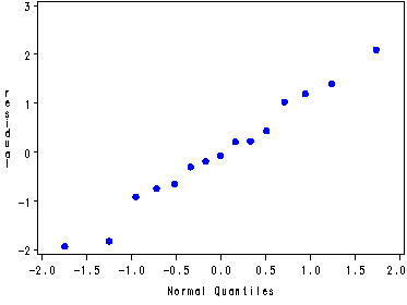
Variance of time by location, bottom of p. 774 and fig. 18.8a and 18.8b, p. 775.

data log;
  set servo;
  logtime = log(time);
run;
proc means data=log var;
  class location;
  var logtime;
run;
quit;
proc glm data=servo noprint;
  class location;
  model time=location;
  output out=temp r=residual;
run;
quit;
goptions reset=all;
symbol1 v=dot c=blue; 
proc capability data=temp noprint;
  qqplot residual;
run;
proc glm data=log noprint;
  class location;
  model logtime=location;
  output out=temp r=residual;
run;
quit;
symbol1 v=dot c=blue; 
proc capability data=temp noprint;
  qqplot residual;
run;

The MEANS Procedure

Analysis Variable : logtime

N
location Obs Variance
———————————–
1 5 1.7420229
2 5 1.9735863
3 5 0.8180583
———————————–

Nonparametric F-test and the Kruskal Wallis test of the Servo data, p. 778-779.

proc npar1way data=servo wilcoxon  anova ;
  class location;
  var time;
  ods output  KruskalWallisTest=temp anova=temp1;
run;
data _null_;
  set temp;
  if label1='Chi-Square' then call symput('chisq', cvalue1);
run;
data _null_;
  set temp1;
  if source='Among' then call symput('between', df);
  if source='Within' then call symput('within', df);
run;
data new;
  fstat = ( &within*&chisq ) / ( &between*(&within+&between - &chisq) );
  fcrit = finv(.9, &between, &within);
  p_value = 1- cdf('F', fstat, &between, &within );
run;
proc print data=new;
run;

The NPAR1WAY Procedure

Analysis of Variance for Variable time
Classified by Variable location

location N Mean
————————————–
1 5 50.3700
2 5 22.1300
3 5 121.2080
Source DF Sum of Squares Mean Square F Value Pr > F
——————————————————————-
Among 2 26053.283213 13026.64161 2.0504 0.1714
Within 12 76238.575080 6353.21459

The NPAR1WAY Procedure

Wilcoxon Scores (Rank Sums) for Variable time
Classified by Variable location

Sum of Expected Std Dev Mean
location N Scores Under H0 Under H0 Score
————————————————————————
1 5 42.0 40.0 8.164966 8.40
2 5 24.0 40.0 8.164966 4.80
3 5 54.0 40.0 8.164966 10.80
Kruskal-Wallis Test
Chi-Square 4.5600
DF 2
Pr > Chi-Square 0.1023
Obs fstat fcrit p_value

1 2.89831 2.80680 0.093986