Applied Linear Statistical Models by Neter, Kutner, et. al. Chapter 20: Analysis of Factor Effects in Two-Factor Studies-Equal Sample Sizes

Inputting the Castle Bakery data, table 19.7, p. 818.

data bakery;
  input sales height width store;
cards;
  47  1  1  1
  43  1  1  2
  46  1  2  1
  40  1  2  2
  62  2  1  1
  68  2  1  2
  67  2  2  1
  71  2  2  2
  41  3  1  1
  39  3  1  2
  42  3  2  1
  46  3  2  2
;
run;

Fig. 20.2, p. 857.
Note: The normal option with mean (mu) and standard deviation (sigma) specified will create the reference line.
When specifying est for either mean or standard deviation or both SAS will estimate the best fit based on the
data.

ods listing close;
proc glm data=bakery;
  class height width;
  model sales = height width height*width;
  means height width;
  ods output means = temp;
run;
quit;
ods listing;
ods output close;
goptions reset=all;
symbol1 c=blue v=dot h=.8;
proc capability data=temp noprint;
  where effect = 'height';
  qqplot  Mean_sales / normal(mu=51 sigma=3);
run;
axis1 order=(40 to 70 by 10);
symbol1 v=dot c=blue h=.8;
proc capability data=temp noprint;
  where effect = 'width';
  qqplot  Mean_sales / vaxis=axis1 normal(mu=est sigma=est);
run;

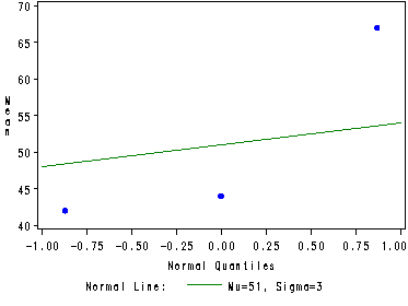
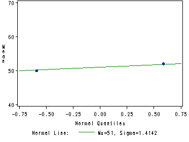
Table 20.1 and confidence intervals for main effects of height and for
the interaction effects, p. 858-859.
Note: Even though we are only interested in the pair-wise tests and the various confidence intervals when we use
proc glm we get a great deal more results in the output. We are interested in the results of the lsmeans
statements and these are located at the end of the output. The results that were calculated in the book are
italicized.

proc glm data=bakery;
  class height width;
  model sales = height width height*width;
  lsmeans height / pdiff adjust=tukey  cl;
  lsmeans height*width / cl;
run;
quit;

The GLM Procedure

Class Level Information

Class Levels Values
height 3 1 2 3
width 2 1 2

Number of observations 12

The GLM Procedure

Dependent Variable: sales
Sum of
Source DF Squares Mean Square F Value Pr > F
Model 5 1580.000000 316.000000 30.58 0.0003
Error 6 62.000000 10.333333
Corrected Total 11 1642.000000
R-Square Coeff Var Root MSE sales Mean
0.962241 6.303040 3.214550 51.00000
Source DF Type I SS Mean Square F Value Pr > F
height 2 1544.000000 772.000000 74.71 <.0001
width 1 12.000000 12.000000 1.16 0.3226
height*width 2 24.000000 12.000000 1.16 0.3747
Source DF Type III SS Mean Square F Value Pr > F
height 2 1544.000000 772.000000 74.71 <.0001
width 1 12.000000 12.000000 1.16 0.3226
height*width 2 24.000000 12.000000 1.16 0.3747

The GLM Procedure
Least Squares Means
Adjustment for Multiple Comparisons: Tukey

LSMEAN
height sales LSMEAN Number
1 44.0000000 1
2 67.0000000 2
3 42.0000000 3
Least Squares Means for effect height
Pr > |t| for H0: LSMean(i)=LSMean(j)

Dependent Variable: sales

i/j 1 2 3
1 0.0001 0.6714
2 0.0001 <.0001
3 0.6714 <.000
height sales LSMEAN 95% Confidence Limits
1 44.000000 40.067139 47.932861
2 67.000000 63.067139 70.932861
3 42.000000 38.067139 45.932861
Least Squares Means for Effect height

Difference Simultaneous 95%
Between Confidence Limits for
i j Means LSMean(i)-LSMean(j)
1 2 -23.000000 -29.973998 -16.026002
1 3 2.000000 -4.973998 8.973998
2 3 25.000000 18.026002 31.973998

The GLM Procedure
Least Squares Means

height width sales LSMEAN
1 1 45.0000000
1 2 43.0000000
2 1 65.0000000
2 2 69.0000000
3 1 40.0000000
3 2 44.0000000
height width sales LSMEAN 95% Confidence Limits
1 1 45.000000 39.438095 50.561905
1 2 43.000000 37.438095 48.561905
2 1 65.000000 59.438095 70.561905
2 2 69.000000 63.438095 74.561905
3 1 40.000000 34.438095 45.561905
3 2 44.000000 38.438095 49.561905

Table 20.3, p. 826.

data burr;
  input efficiency spacing speed;
cards;
  21.6  1.0  300
  22.3  1.0  400
  22.9  1.0  500
  18.7  1.2  300
  19.1  1.2  400
  21.6  1.2  500
  15.8  1.4  300
  17.9  1.4  400
  19.4  1.4  500
  13.2  1.6  300
  16.7  1.6  400
  19.5  1.6  500
;
run;

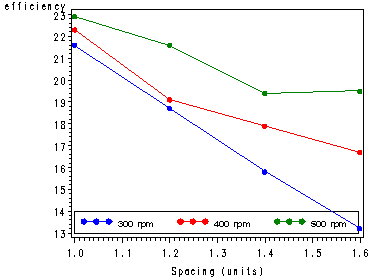
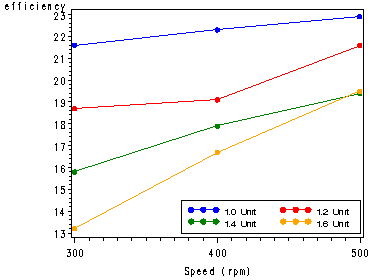
Fig. 20.5, p. 867.
Note: In order to get the lines on the same graph we need to create three variables for spacing that corresponds
to each of the levels of speed. Likewise, we create four variables for speed corresponding to each of the
levels for spacing. The overlay option in the plot statement lets us plot all the lines in the same
graph.

data burr;
  set burr;
  if speed = 300 then rpm300 = spacing;
  if speed = 400 then rpm400 = spacing;
  if speed = 500 then rpm500 = spacing;
  if spacing = 1 then spac1 = speed;
  if spacing = 1.2 then spac12 = speed;
  if spacing = 1.4 then spac14 = speed;
  if spacing = 1.6 then spac16 = speed;
run;
goptions reset = all;
symbol1 v=dot c=blue h=.8 i=join;
symbol2 v=dot c=red h=.8 i=join;
symbol3 v=dot c=green h=.8 i=join;
symbol4 v=dot c=orange h=.8 i=join;
legend1 label=none value=(height=1 font=swiss '300 rpm' '400 rpm' '500 rpm' ) 
        position=(left bottom  inside) mode=share cborder=black;
axis1 label=('Spacing (units)');
legend2 label=none value=(height=1 font=swiss '1.0 Unit' '1.2 Unit' '1.4 Unit' '1.6 Unit' ) 
        position=(right bottom  inside) mode=share cborder=black;
axis2 label=('Speed (rpm)');
proc gplot data=burr;
  plot efficiency*(rpm300 rpm400 rpm500) / overlay legend=legend1 haxis=axis1;
  plot efficiency*(spac1 spac12 spac14 spac16) / overlay legend=legend2 haxis=axis2;
run;
quit;
goptions reset=all;