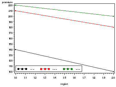
Applied Linear Statistical Models by Neter, Kutner, et. al. Chapter 21: Two-Factor Studies–One Case Per Treatment

Inputting the Insurance Premium data, table 21.2a, p. 878. The proc glm was used to produce the ANOVA table. The means statement generated the means of premium for each level of of city and each level of region, table 21.2b, p. 878. The output from proc glm also includes the F-tests of each predictor, p. 879-880.

data insurance;
  input premium city region;
cards;
  140  1  1
  100  1  2
  210  2  1
  180  2  2
  220  3  1
  200  3  2
;
run;
proc glm data=insurance;
  class city region;
  model premium = city region;
  means city region;
run;
quit;

The GLM Procedure

Class Level Information

Class Levels Values city 3 1 2 3 region 2 1 2

Number of observations 6

The GLM Procedure

Dependent Variable: premium Sum of Source DF Squares Mean Square F Value Pr > F Model 3 10650.00000 3550.00000 71.00 0.0139 Error 2 100.00000 50.00000 Corrected Total 5 10750.00000 R-Square Coeff Var Root MSE premium Mean 0.990698 4.040610 7.071068 175.0000 Source DF Type I SS Mean Square F Value Pr > F city 2 9300.000000 4650.000000 93.00 0.0106 region 1 1350.000000 1350.000000 27.00 0.0351 Source DF Type III SS Mean Square F Value Pr > F city 2 9300.000000 4650.000000 93.00 0.0106 region 1 1350.000000 1350.000000 27.00 0.0351

The GLM Procedure

Level of ———–premium———– city N Mean Std Dev 1 2 120.000000 28.2842712 2 2 195.000000 21.2132034 3 2 210.000000 14.1421356

Level of ———–premium———– region N Mean Std Dev 1 3 190.000000 43.5889894 2 3 160.000000 52.9150262

Fig. 21.1, p. 879.
In order to get the lines in the same graph we need to create three variables for region that corresponds to each of the levels of city. The overlay option in the plot statement lets us plot all the lines in the same graph.

symbol v=dot i=join;
legend1 label=none value=(height=1 font=swiss 'Large City' 'Medium City' 'Small City' ) 
        position=(left bottom  inside) mode=share cborder=black;
proc gplot data=insurance;
plot premium*region=city /legend=legend1;
run;
quit;

Predicting estimates of the treatment means, p. 881.

proc glm data=insurance noprint;
  class city region;
  model premium = city region ;
  output out=temp p=predict;
run;
quit;
proc print data=temp;
 var city region premium predict;
run;

Obs city region premium predict

1 1 1 140 135 2 1 2 100 105 3 2 1 210 210 4 2 2 180 180 5 3 1 220 225 6 3 2 200 195

Creating the dummy variables for city and region, p. 881. Running the regression to get the factor effects alphai and betaj. When looking at the predict values from the regression we see that we get exactly the same values as from the proc glm.

data dummy;
  set insurance;
  if city=1 then x1=1;
  else if city=3 then x1=-1;
  else x1=0;
  if city=2 then x2=1;
  else if city=3 then x2=-1;
  else x2=0;
  if region=1 then x3=1;
  else x3=-1;
run;
proc reg data=dummy;
  model premium = x1 x2 x3;
  output out=temp p=predict;
run;
quit;
proc print data=temp;
  var city region premium predict;
run;

The REG Procedure Model: MODEL1 Dependent Variable: premium

Analysis of Variance

Sum of Mean Source DF Squares Square F Value Pr > F Model 3 10650 3550.00000 71.00 0.0139 Error 2 100.00000 50.00000 Corrected Total 5 10750

Root MSE 7.07107 R-Square 0.9907 Dependent Mean 175.00000 Adj R-Sq 0.9767 Coeff Var 4.04061 Parameter Estimates

Parameter Standard Variable DF Estimate Error t Value Pr > |t| Intercept 1 175.00000 2.88675 60.62 0.0003 x1 1 -55.00000 4.08248 -13.47 0.0055 x2 1 20.00000 4.08248 4.90 0.0392 x3 1 15.00000 2.88675 5.20 0.0351 Obs city region premium predict

1 1 1 140 135 2 1 2 100 105 3 2 1 210 210 4 2 2 180 180 5 3 1 220 225 6 3 2 200 195

Tukey test of Additivity for the insurance data, p. 884.
We need to obtain the sums of squares for each predictor and the corrected total sums of squares which is most easily accomplished using the ODS system and then saved as macro variables. Using the macro variables and several sql procedures we can then create the SSAB, SSrem values and the F test in a data step at the end of the program.

ods listing close;
proc glm data=insurance;
  class region city;
  model premium = region city;
  ods output overallanova=overall modelanova=model;
run;
quit;
ods listing;
ods output close;
data _null_;
  set overall;
  if source='Corrected Total' then call symput('overall', ss);
run;
data _null_;
  set model ;
  if hypothesistype=1 and source='city' then call symput('ssa', ss);
  if hypothesistype=1 and source='region' then call symput('ssb', ss);
  if hypothesistype=1 and source='city' then call symput('dfa', df);
  if hypothesistype=1 and source='region' then call symput('dfb', df);
run;
%put here is &overall &ssa &ssb &dfa &dfb; /* the statement will appear in the log file so you can check the calculations */
proc sql;
  create table temp1 as
  select premium, region, city , mean(premium) as yj
  from insurance
  group by region;
quit;
proc sql;
  create table temp2 as
  select *, mean(premium) as yi
  from temp1
  group by city;
quit;
proc sql noprint; 
   select mean(premium) into :meanp from temp1;
quit;
%put here is  &meanp; /* check value in log file */
proc sql noprint;
  select sum( (yi - &meanp)*(yj - &meanp)*premium ) into :total from temp2;
quit;
%put here is &total; /*check value in log file*/
data final;
  msa = &ssa/(&dfb+1);
  msb = &ssb/(&dfa+1);
  ssab = (&total*&total) / ( msa*msb );
  ssrem = &overall - &ssa - &ssb - ssab;
  f = ssab/( ssrem/((&dfa+1)*(&dfb+1) - (&dfa+1) - (&dfb+1)) );
  p_value = 1- cdf('F',f,  1, (&dfa+1)*(&dfb+1) - (&dfa+1) - (&dfb+1) );
run;
proc print data=final;
run;

Obs     msa    msb      ssab      ssrem       f     p_value
 1     4650    450    87.0968    12.9032    6.75    0.23391