Applied Linear Statistical Models by Neter, Kutner, et. al. Chapter 22: Two-Factor Studies–Unequal Sample Sizes and Unequal Treatment Importance

Inputting the Growth Hormone data and computing the factor level means, table 22.1, p. 892.

data growth;
  input growth gender depress rep;
cards;
  1.4  1  1  1
  2.4  1  1  2
  2.2  1  1  3
  2.1  1  2  1
  1.7  1  2  2
  0.7  1  3  1
  1.1  1  3  2
  2.4  2  1  1
  2.5  2  2  1
  1.8  2  2  2
  2.0  2  2  3
  0.5  2  3  1
  0.9  2  3  2
  1.3  2  3  3
;
run;
proc means data=growth mean;
  class gender depress ;
  var growth;
run;

The MEANS Procedure

Analysis Variable : growth

N
gender depress Obs Mean
—————————————————
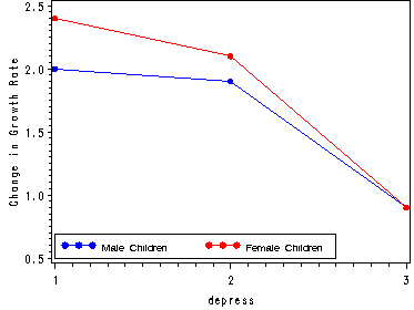
1 1 3 2.0000000
2 2 1.9000000
3 2 0.9000000
2 1 1 2.4000000
2 3 2.1000000
3 3 0.9000000
—————————————————

Fig. 22.1, p. 892.

Note: We create two variables for depression means, one for each level of gender. The overlay option in
proc gplot lets us plot the two lines in the same graph.

proc means data=growth mean noprint;
  class gender depress;
  var growth;
  output out=temp mean=mout;
run; 
data temp;
  set temp;
  if gender=1 then male=mout;
  if gender=2 then female=mout;
run;
goptions reset=all;
 
symbol1 c=blue v=dot h=.8 i=join;
symbol2 c=red v=dot h=.8 i=join;
axis1 order=(.5 to 2.5 by .5) label=(angle=90 'Change in Growth Rate');
legend1 label=none value=(height=1 font=swiss 'Male Children' 'Female Children' ) 
        position=(left bottom inside) mode=share cborder=black;
proc gplot data=temp;
  plot (male female)*depress/ overlay legend=legend1 vaxis=axis;
run;
quit;

Creating the dummy variables to be used in the regression model that will be equivalent to
the ANOVA model (22.3), p. 893.

data dummy;
  set growth;
  if gender=1 then x1=1;
  else x1=-1;
  if depress=1 then x2=1;
  else if depress=3 then x2=-1;
  else x2=0;
  if depress=2 then x3=1;
  else if depress=3 then x3=-1;
  else x3=0;
  x1x2 = x1*x2;
  x1x3 = x1*x3;
run;

Table 22.2, p. 894.

proc print data=dummy;
  var gender depress rep growth x1 x2 x3 x1x2 x1x3;
run;

Obs    gender    depress    rep    growth    x1    x2    x3    x1x2    x1x3

  1       1         1        1       1.4      1     1     0      1       0

  2       1         1        2       2.4      1     1     0      1       0

  3       1         1        3       2.2      1     1     0      1       0

  4       1         2        1       2.1      1     0     1      0       1

  5       1         2        2       1.7      1     0     1      0       1

  6       1         3        1       0.7      1    -1    -1     -1      -1

  7       1         3        2       1.1      1    -1    -1     -1      -1

  8       2         1        1       2.4     -1     1     0     -1       0

  9       2         2        1       2.5     -1     0     1      0      -1

 10       2         2        2       1.8     -1     0     1      0      -1

 11       2         2        3       2.0     -1     0     1      0      -1

 12       2         3        1       0.5     -1    -1    -1      1       1

 13       2         3        2       0.9     -1    -1    -1      1       1

 14       2         3        3       1.3     -1    -1    -1      1       1

Table 22.3, p. 895.

proc reg data=dummy;
  model growth = x1 x2 x3 x1x2 x1x3;
  model growth = x1 x2 x3;
  model growth = x2 x3 x1x2 x1x3;
  model growth = x1 x1x2 x1x3; 
run;
quit;

The REG Procedure
Model: MODEL1
Dependent Variable: growth

Analysis of Variance

Sum of Mean
Source DF Squares Square F Value Pr > F
Model 5 4.47429 0.89486 5.51 0.0172
Error 8 1.30000 0.16250
Corrected Total 13 5.77429

Root MSE 0.40311 R-Square 0.7749
Dependent Mean 1.64286 Adj R-Sq 0.6342
Coeff Var 24.53731
Parameter Estimates

Parameter Standard
Variable DF Estimate Error t Value Pr > |t|
Intercept 1 1.70000 0.11637 14.61 <.0001
x1 1 -0.10000 0.11637 -0.86 0.4152
x2 1 0.50000 0.17776 2.81 0.0227
x3 1 0.30000 0.15756 1.90 0.0934
x1x2 1 -0.10000 0.17776 -0.56 0.5891
x1x3 1 -4.8512E-17 0.15756 -0.00 1.0000

The REG Procedure
Model: MODEL2
Dependent Variable: growth

Analysis of Variance

Sum of Mean
Source DF Squares Square F Value Pr > F
Model 3 4.39886 1.46629 10.66 0.0019
Error 10 1.37543 0.13754
Corrected Total 13 5.77429

Root MSE 0.37087 R-Square 0.7618
Dependent Mean 1.64286 Adj R-Sq 0.6903
Coeff Var 22.57456
Parameter Estimates

Parameter Standard
Variable DF Estimate Error t Value Pr > |t|
Intercept 1 1.67619 0.09973 16.81 <.0001
x1 1 -0.08571 0.10448 -0.82 0.4311
x2 1 0.46667 0.15418 3.03 0.0127
x3 1 0.32667 0.14035 2.33 0.0422

The REG Procedure
Model: MODEL3
Dependent Variable: growth

Analysis of Variance

Sum of Mean
Source DF Squares Square F Value Pr > F
Model 4 4.35429 1.08857 6.90 0.0080
Error 9 1.42000 0.15778
Corrected Total 13 5.77429

Root MSE 0.39721 R-Square 0.7541
Dependent Mean 1.64286 Adj R-Sq 0.6448
Coeff Var 24.17815
Parameter Estimates

Parameter Standard
Variable DF Estimate Error t Value Pr > |t|
Intercept 1 1.68889 0.11396 14.82 <.0001
x2 1 0.44444 0.16316 2.72 0.0235
x3 1 0.32778 0.15196 2.16 0.0594
x1x2 1 -0.06667 0.17093 -0.39 0.7056
x1x3 1 -0.01667 0.15408 -0.11 0.9162

The REG Procedure
Model: MODEL4
Dependent Variable: growth

Analysis of Variance

Sum of Mean
Source DF Squares Square F Value Pr > F
Model 3 0.28457 0.09486 0.17 0.9124
Error 10 5.48971 0.54897
Corrected Total 13 5.77429

Root MSE 0.74093 R-Square 0.0493
Dependent Mean 1.64286 Adj R-Sq -0.2359
Coeff Var 45.09985
Parameter Estimates

Parameter Standard
Variable DF Estimate Error t Value Pr > |t|
Intercept 1 1.62857 0.20873 7.80 <.0001
x1 1 0.01905 0.19924 0.10 0.9257
x1x2 1 0.06667 0.30803 0.22 0.8330
x1x3 1 -0.19333 0.28039 -0.69 0.5062

Testing the interactions, factor A main effects and factor B main effects, p. 894-896.

proc reg data=dummy;
  model growth = x1 x2 x3 x1x2 x1x3;
  interactions: test x1x2, x1x3;
  maina: test x1;
  mainb: test x2, x3;
run;
quit;

The REG Procedure
Model: MODEL1
Dependent Variable: growth

                             Analysis of Variance

                                    Sum of           Mean
Source                   DF        Squares         Square    F Value    Pr > F

Model                     5        4.47429        0.89486       5.51    0.0172
Error                     8        1.30000        0.16250
Corrected Total          13        5.77429

Root MSE              0.40311    R-Square     0.7749
Dependent Mean        1.64286    Adj R-Sq     0.6342
Coeff Var            24.53731

                        Parameter Estimates

                     Parameter       Standard
Variable     DF       Estimate          Error    t Value    Pr > |t|

Intercept     1        1.70000        0.11637      14.61      <.0001
x1            1       -0.10000        0.11637      -0.86      0.4152
x2            1        0.50000        0.17776       2.81      0.0227
x3            1        0.30000        0.15756       1.90      0.0934
x1x2          1       -0.10000        0.17776      -0.56      0.5891
x1x3          1    -4.8512E-17        0.15756      -0.00      1.0000

The REG Procedure
Model: MODEL1

 Test interactions Results for Dependent Variable growth

                                Mean
Source             DF         Square    F Value    Pr > F

Numerator           2        0.03771       0.23    0.7980
Denominator         8        0.16250

The REG Procedure
Model: MODEL1

    Test maina Results for Dependent Variable growth

                                Mean
Source             DF         Square    F Value    Pr > F

Numerator           1        0.12000       0.74    0.4152
Denominator         8        0.16250

The REG Procedure
Model: MODEL1

    Test mainb Results for Dependent Variable growth

                                Mean
Source             DF         Square    F Value    Pr > F

Numerator           2        2.09486      12.89    0.0031
Denominator         8        0.16250

Table 22.4, p. 897.

proc glm data=growth;
  class gender depress;
  model growth = gender depress gender*depress/ss3;
run;
quit;

The GLM Procedure

Class Level Information

Class Levels Values
gender 2 1 2
depress 3 1 2 3

Number of observations 14

The GLM Procedure

Dependent Variable: growth

Sum of
Source DF Squares Mean Square F Value Pr > F
Model 5 4.47428571 0.89485714 5.51 0.0172
Error 8 1.30000000 0.16250000
Corrected Total 13 5.77428571

R-Square Coeff Var Root MSE growth Mean
0.774864 24.53731 0.403113 1.642857
Source DF Type III SS Mean Square F Value Pr > F
gender 1 0.12000000 0.12000000 0.74 0.4152
depress 2 4.18971429 2.09485714 12.89 0.0031
gender*depress 2 0.07542857 0.03771429 0.23 0.7980

Pair-wise comparisons of depress factor level means, p. 901.
Note: Since the model is the same as above all the redundant output has been omitted.

proc glm data=growth;
  class depress gender;
  model growth = depress gender depress*gender;
  lsmeans depress/ pdiff adjust=tukey cl alpha=.1;
run;
quit;

The GLM Procedure
<output omitted>
Least Squares Means

Adjustment for Multiple Comparisons: Tukey-Kramer
                 growth      LSMEAN

depress          LSMEAN      Number
1            2.20000000           1

2            2.00000000           2

3            0.90000000           3
    Least Squares Means for effect depress

     Pr > |t| for H0: LSMean(i)=LSMean(j)
          Dependent Variable: growth
i/j              1             2             3
   1                      0.7845        0.0059

   2        0.7845                      0.0072

   3        0.0059        0.0072
                 growth

depress          LSMEAN      90% Confidence Limits
1              2.200000        1.767214     2.632786

2              2.000000        1.657852     2.342148

3              0.900000        0.557852     1.242148
       Least Squares Means for Effect depress
            Difference         Simultaneous 90%

               Between      Confidence Limits for

i    j           Means       LSMean(i)-LSMean(j)
1    2        0.200000       -0.507807     0.907807

1    3        1.300000        0.592193     2.007807

2    3        1.100000        0.479212     1.720788
Single degree of Freedom test using the growth hormone example, p. 902. 
 

Note: The single degree t-tests are obtained by using the lsmeans statement with the tdiff option.

Moreover, since the model is the same as in the two previous proc glm the redundant output has been omitted.
proc glm data=growth;
  class  depress gender;
  model growth = depress gender depress*gender;
  lsmeans depress/ tdiff stderr;
run;
quit;
<output omitted>

The GLM Procedure
Least Squares Means

                 growth        Standard                  LSMEAN
depress          LSMEAN           Error    Pr > |t|      Number

1            2.20000000      0.23273733      <.0001           1
2            2.00000000      0.18399502      <.0001           2
3            0.90000000      0.18399502      0.0012           3

    Least Squares Means for Effect depress
   t for H0: LSMean(i)=LSMean(j) / Pr > |t|

          Dependent Variable: growth

i/j              1             2             3

   1                     0.67412       4.38178
                          0.5192        0.0023
   2      -0.67412                    4.227383
            0.5192                      0.0029
   3      -4.38178      -4.22738
            0.0023        0.0029

NOTE: To ensure overall protection level, only probabilities associated with pre-planned
      comparisons should be used.
We cannot reproduce the math score example since the data was not available, p. 906.
Tests of the null hypothesis in (22.24a) first using proc glm and then using two regression models, p. 907-908.


Note: In the code for proc glm the order of the categorical

variables in the class statement is very important and it has to match the order to the

interaction.  If the interaction is gender*depress then the class statement has

to be class gender depress. It is rather tricky figuring out the order of the coefficients

that should be entered into the contrast statement.  When the interaction is gender*depress

the coefficients in the contrast statement are those of the cell means in the following order:

mu11 mu12 mu13 mu21 mu22 mu23 where the first index is for the gender factor and the second index

is for the depress factor.  In the second version of the code where the order of the interaction

was switched the coefficients in the contrast statement are those of the cell means in the following

order:  mu11 mu21 mu12 mu22 mu13 mu23 (where the first index is for the gender factor and the second index

is for the depress factor).
proc glm data=growth;
  class gender depress;
  model growth =  gender*depress;
  contrast 'contrast'
    gender*depress .666 -.666 0 .333 -.333 0,
    gender*depress .666 0 -.666 .333 0 -.333;       
run;
quit;
proc glm data=growth;
  class  depress gender ;
  model growth =  depress*gender;
  contrast 'contrast'
    depress*gender .666 .333 -.666 -.333 0 0,
    depress*gender .666  .333 0 0  -.666 -.333;       
run;
quit;
The GLM Procedure
   Class Level Information
Class         Levels    Values

gender             2    1 2

depress            3    1 2 3
Number of observations    14
The GLM Procedure

Dependent Variable: growth
                                        Sum of

Source                      DF         Squares     Mean Square    F Value    Pr > F
Model                        5      4.47428571      0.89485714       5.51    0.0172

Error                        8      1.30000000      0.16250000

Corrected Total             13      5.77428571

R-Square     Coeff Var      Root MSE    growth Mean
0.774864      24.53731      0.403113       1.642857
Source                      DF       Type I SS     Mean Square    F Value    Pr > F

gender*depress               5      4.47428571      0.89485714       5.51    0.0172

Source                      DF     Type III SS     Mean Square    F Value    Pr > F

gender*depress               5      4.47428571      0.89485714       5.51    0.0172
Contrast                    DF     Contrast SS     Mean Square    F Value    Pr > F

contrast                     2      3.45428571      1.72714286      10.63    0.0056
The GLM Procedure
   Class Level Information
Class         Levels    Values

depress            3    1 2 3

gender             2    1 2
Number of observations    14
The GLM Procedure

Dependent Variable: growth
                                        Sum of

Source                      DF         Squares     Mean Square    F Value    Pr > F
Model                        5      4.47428571      0.89485714       5.51    0.0172

Error                        8      1.30000000      0.16250000

Corrected Total             13      5.77428571
R-Square     Coeff Var      Root MSE    growth Mean

0.774864      24.53731      0.403113       1.642857
Source                      DF       Type I SS     Mean Square    F Value    Pr > F

depress*gender               5      4.47428571      0.89485714       5.51    0.0172
Source                      DF     Type III SS     Mean Square    F Value    Pr > F

depress*gender               5      4.47428571      0.89485714       5.51    0.0172

Contrast                    DF     Contrast SS     Mean Square    F Value    Pr > F

contrast                     2      3.45428571      1.72714286      10.63    0.0056

Creating the dummy variables to get the regression model that will supply us with the value of

SSE(F), p. 908.
data dummyx;
  set growth;
  x1 = 0;
  if gender=1 and depress=1 then x1=1;
  x2 = 0;
  if gender=1 and depress=2 then x2=1;
  x3 = 0;
  if gender=1 and depress=3 then x3=1;
  x4 = 0;
  if gender=2 and depress=1 then x4=1;
  x5 = 0;
  if gender=2 and depress=2 then x5=1;
  x6 = 0;
  if gender=2 and depress=3 then x6=1;
run;
Running the regression model and using ODS to create two macro variables, one for SSE(F) and

one for DF_F. In order to check that we have the correct macro variable we use a put statement

to look at the macro variables in the log file.
ods listing close;
ods output anova=full;
proc reg data = dummyx;
  model growth = x1-x6 / noint;
run;
quit;
ods listing;
data _null_;
  set full;
  if source='Error' then call symput('fullss', ss);
  if source='Error' then call symput('fulldf', df);
run;
%put here are the values &fullss and &fulldf; /* check values in the log file */ 
Creating the dummy variables for the reduced regression model, p. 909 and running the second

regression model and using ODS to create two macro variables, one for SSE(R) and one for DF_R. In order to

check that we have the correct macro variable we use a put statement

to look at the macro variables in the log file.
data dummyz;
  set dummyx;
  z1 = x1 - 2*x4;
  z2 = x2 +2*x4 +2*x6;
  z3 = x3 -2*x6;
  z4 = x4 +x5+x6;
run;
ods listing close;
ods output anova=reduced;
proc reg data=dummyz;
  model growth = z1-z4/ noint;
run;
quit;
ods listing;
data _null_;
  set reduced;
  if source='Error' then call symput('reducedss', ss);
  if source='Error' then call symput('reduceddf', df);
run;
%put here are the values &reducedss and &reduceddf; /* check values in log file */
Finally, we use all the values that were extracted from the two regression models in an F-test, p. 909.
data temp;
  SSE_R= &reducedss;
  SSE_F= &fullss;
  DF_R = &reduceddf;
  DF_F = &fulldf;
  Fstar = ( (&reducess - &fullss)/( &reduceddf - &fulldf) ) /( &fullss/ &fulldf);
  p_value = 1 - cdf( 'F', fstar, &reduceddf - &fulldf, &fulldf);
run;
proc print data=temp;
run;
Obs     SSE_R     SSE_F    DF_R    DF_F     Fstar        p_value
 1     4.75429     1.3      10       8     10.6286    .005590264

Repeating the same test using SSA, p. 914. 
 

Note: First we use proc glm to obtain SSA and the DF_A and store them as macro variables.

Then we will use the data set dummy and re-run the full regression model including interactions in

order to obtain the SSE(F) and df_F as presented in table 22.3a, p. 895 and store them as macro variables.  Finally,

we use all the values that we extracted in an F-test.
ods listing close;
ods output  ModelANOVA=ssa;
proc glm data=growth;
  class gender depress;
  model growth = gender depress/ ss1;
run;
quit;
ods listing;
data _null_;
  set ssa;
  if source='gender' then call symput('ssa', ss);
  if source='gender' then call symput('dfa', df);
run;
%put here are the values &ssa and &dfa; /*check the values in the log file */
ods listing close;
ods output anova=anova;
proc reg data=dummy;
 model growth = x1 x2 x3 x1x2 x1x3;
run;
quit;
ods listing;
data _null_;
  set anova;
  if source='Error' then call symput('fullss', ss);
  if source='Error' then call symput('fulldf', df);
run;
%put here are the values &fullss and &fulldf; /* check the values in the log file */
data temp;
  SSA = &ssa;
  DF_A = &dfa;
  SSE_F = &fullss;
  DF_F = &fulldf;
  Fstar = (&ssa/&dfa)/( &fullss/ &fulldf);
  p_value = 1 - cdf( 'F', Fstar, &dfa, &fulldf);
run;
proc print data=temp;
run;
Obs          SSA     DF_A    SSE_F    DF_F      Fstar     p_value
 1     .002857143      1      1.3       8     0.017582    0.89779