Applied Linear Statistical Models by Neter, Kutner, et. al. Chapter 27: Randomized Block Design

Inputting the Confidence Rating data set, table 27.1, p. 1076.

data confidence;
  input score block treat;
cards;
   1  1  1
   5  1  2
   8  1  3
   2  2  1
   8  2  2
  14  2  3
   7  3  1
   9  3  2
  16  3  3
   6  4  1
  13  4  2
  18  4  3
  12  5  1
  14  5  2
  17  5  3
;
run;

Fig. 27.2, p. 1077.

data plot;
  set confidence;
  if block=1 then b1=score;
  if block=2 then b2=score;
  if block=3 then b3=score;
  if block=4 then b4=score;
  if block=5 then b5=score;
run;
goptions reset=all;
 
symbol1 c=blue v=dot i=join;
symbol2 c=red v=circle i=join;
symbol3 c=green v=triangle i=join;
symbol4 c=purple v=plus i=join;
symbol5 c=cyan v=: i=join;
axis1 order=(0 to 20 by 5) label=(a=90 'Confidence Rating');
axis2 offset=(5,5);
legend1 label=none value=(height=.75 font=swiss 'Block 1' 'Block 2' 'Block 3' 'Block 4' 'Block 5' ) 
        position=(top left inside) mode=share cborder=black;
proc gplot data=plot;
  plot (b1 b2 b3 b4 b5)*treat/ overlay vaxis=axis1 haxis=axis2 legend=legend1;
run;
quit;
goptions reset=all;

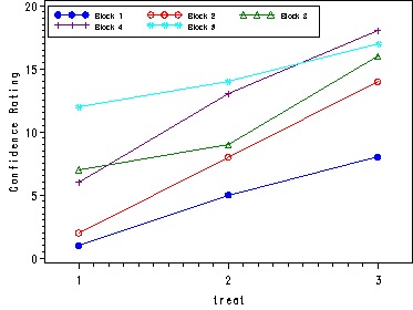
Table 27.3, ANOVA table for Confidence Rating data, p. 1080.

proc glm data=confidence;
  class block treat;
  model score = treat block;
  output out=outglm r=resid p=predict;
run;
quit;

The GLM Procedure

Class Level Information

Class Levels Values
block 5 1 2 3 4 5
treat 3 1 2 3

Number of observations 15
The GLM Procedure
Dependent Variable: score
Sum of
Source DF Squares Mean Square F Value Pr > F
Model 6 374.1333333 62.3555556 20.90 0.0002
Error 8 23.8666667 2.9833333
Corrected Total 14 398.0000000

R-Square Coeff Var Root MSE score Mean
0.940034 17.27233 1.727233 10.00000

Source DF Type I SS Mean Square F Value Pr > F
treat 2 202.8000000 101.4000000 33.99 0.0001
block 4 171.3333333 42.8333333 14.36 0.0010
Source DF Type III SS Mean Square F Value Pr > F
treat 2 202.8000000 101.4000000 33.99 0.0001
block 4 171.3333333 42.8333333 14.36 0.0010

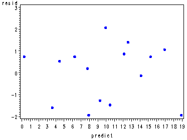
Fig. 27.5, Residual plot, p. 1083.


symbol v=dot c=blue h=.8;
proc gplot data=outglm;
  plot resid*predict;
run;
quit;
proc capability data=outglm noprint;
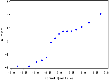
  qqplot resid;
run;

Testing if there is an interaction between blocks and treatment, p. 1083-1084.

ods listing close;
proc glm data=confidence;
  class block treat;
  model score = treat block;
  ods output overallanova=overall modelanova=model;
run;
quit;
ods listing;
ods output close;
data _null_;
  set overall;
  if source='Corrected Total' then call symput('overall', ss);
run;
data _null_;
  set model ;
  if hypothesistype=1 and source='treat' then call symput('sstr', ss);
  if hypothesistype=1 and source='block' then call symput('ssbk', ss);
  if hypothesistype=1 and source='treat' then call symput('dftr', df);
  if hypothesistype=1 and source='block' then call symput('dfbk', df);
run;
%put they here are &overall &sstr &ssbk &dftr &dfbk; /*check numbers in log file*/
proc sql;
  create table temp1 as
  select score, block, treat , mean(score) as yj
  from confidence
  group by block;
quit;
proc sql noprint;
  create table temp2 as
  select *, mean(score) as yi
  from temp1
  group by treat;
quit;
proc sql noprint; 
   select mean(score) into :meanp from temp1;
quit;
%put here is the grand mean = &meanp; /*check numbers in log file*/
proc sql noprint;
  select  sum( (yi - 10)*(yj-10)*score ) into :total
  from temp2;
quit;
%put here is &total; /*check numbers in log file*/
data final;
  msa = &sstr/(&dftr+1);
  msb = &ssbk/(&dfbk+1);
  sstr_bk = (&total*&total) / ( msa*msb );
  ssrem = &overall - &sstr - &ssbk - sstr_bk;
  f = sstr_bk/( ssrem/((&dftr+1)*(&dfbk+1) - (&dftr+1) - (&dfbk+1)) );
  p_value = 1- cdf('F',f,  1, (&dftr+1)*(&dfbk+1) - (&dftr+1) - (&dfbk+1) );
run;
proc print data=final;
run;

Obs msa msb sstr_bk ssrem f p_value

1 67.6 34.2667 0.26267 23.6040 0.077896 0.78823

Pairwise comparisons using the Tukey procedure and a 95% family confidence coefficient, p. 1086.

proc glm data=confidence;
  class block treat;
  model score=block treat;
  lsmeans treat/ cl adjust=tukey pdiff;
  ods output lsmeans=temp;
run;
quit;

The GLM Procedure

Class Level Information

Class Levels Values
block 5 1 2 3 4 5
treat 3 1 2 3

Number of observations 15

The GLM Procedure
Dependent Variable: score
Sum of
Source DF Squares Mean Square F Value Pr > F
Model 6 374.1333333 62.3555556 20.90 0.0002
Error 8 23.8666667 2.9833333
Corrected Total 14 398.0000000

R-Square Coeff Var Root MSE score Mean
0.940034 17.27233 1.727233 10.00000

Source DF Type I SS Mean Square F Value Pr > F
block 4 171.3333333 42.8333333 14.36 0.0010
treat 2 202.8000000 101.4000000 33.99 0.0001
Source DF Type III SS Mean Square F Value Pr > F
block 4 171.3333333 42.8333333 14.36 0.0010
treat 2 202.8000000 101.4000000 33.99 0.0001

The GLM Procedure
Least Squares Means
Adjustment for Multiple Comparisons: Tukey
LSMEAN
treat score LSMEAN Number
1 5.6000000 1
2 9.8000000 2
3 14.6000000 3

Least Squares Means for effect treat
Pr > |t| for H0: LSMean(i)=LSMean(j)

Dependent Variable: score
i/j 1 2 3
1 0.0121 <.0001
2 0.0121 0.0058
3 <.0001 0.0058

treat score LSMEAN 95% Confidence Limits
1 5.600000 3.818746 7.381254
2 9.800000 8.018746 11.581254
3 14.600000 12.818746 16.381254

Least Squares Means for Effect treat

Difference Simultaneous 95%
Between Confidence Limits for
i j Means LSMean(i)-LSMean(j)
1 2 -4.200000 -7.321443 -1.078557
1 3 -9.000000 -12.121443 -5.878557
2 3 -4.800000 -7.921443 -1.678557

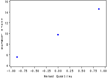
Fig. 17.4, p. 728.

goptions reset=all;
symbol v=dot c=blue h=.8;
proc capability data=temp noprint;
  qqplot LSMean;
run;
quit;

Evaluating the efficiency of blocking by age of executives in the Confidence Rating, p. 1090.

ods listing close;
proc glm data=confidence;
  class block treat;
  model score = treat block;
  ods output overallanova=overall modelanova=model;
run;
quit;
ods listing;
ods output close;
data _null_;
  set model ;
  if hypothesistype=1 and source='block' then call symput('msbk', ms);
  if hypothesistype=1 and source='treat' then call symput('dftr', df);
  if hypothesistype=1 and source='block' then call symput('dfbk', df);
run;
%put they here are &msbk  &dftr &dfbk; /*check numbers in log file*/
data _null_;
  set overall;
  if source='Error' then call symput('mse', ms);
  if source='Error' then call symput('dfe', df);
run;
%put they here are &mse &dfe; /*check numbers in log file*/
data temp;
  Ehat = (&dfbk*&msbk + (&dfbk+1)*&dftr*&mse )/( ((&dfbk+1)*(&dftr+1) - 1)*&mse );
  Eprime = (((&dfe+1)*(12+3))/( (&dfe+3)*(12+1)))*Ehat;
run;
proc print data=temp;
run;

Obs Ehat Eprime

1 4.81644 4.54699

Regression approach to randomized block design. Generating the appropriate variables when
applying deviation coding to both the block variable and the treatment variable, table 27.5, p. 1092.

Note: For more information on deviation coding please refer to chapter 5 in our webbook at
https://stats.idre.ucla.edu/stat/sas/webbooks/reg/chapter5/sasreg5.htm
.

data reg;
  set confidence;
  x1 =0;
  if block=1 then x1=1;
  else if block=5 then x1=-1;
  x2 =0;
  if block=2 then x2=1;
  else if block=5 then x2=-1;
  x3 =0;
  if block=3 then x3=1;
  else if block=5 then x3=-1;
  x4 =0;
  if block=4 then x4=1;
  else if block=5 then x4=-1;
  x5=0;
  if treat=1 then x5=1;
  else if treat=3 then x5=-1;
  x6=0;
  if treat=2 then x6=1;
  else if treat=3 then x6=-1;
run;
proc reg data=reg;
  model score = x1-x6;
  block: test x1=x2=x3=x4=0;
  treatment: test x5=x6=0;
run;
quit;

The REG Procedure
Model: MODEL1
Dependent Variable: score

Analysis of Variance

Sum of Mean
Source DF Squares Square F Value Pr > F
Model 6 374.13333 62.35556 20.90 0.0002
Error 8 23.86667 2.98333
Corrected Total 14 398.00000

Root MSE 1.72723 R-Square 0.9400
Dependent Mean 10.00000 Adj R-Sq 0.8951
Coeff Var 17.27233

Parameter Estimates

Parameter Standard
Variable DF Estimate Error t Value Pr > |t
Intercept 1 10.00000 0.44597 22.42 <.0001
x1 1 -5.33333 0.89194 -5.98 0.0003
x2 1 -2.00000 0.89194 -2.24 0.0552
x3 1 0.66667 0.89194 0.75 0.4762
x4 1 2.33333 0.89194 2.62 0.0308
x5 1 -4.40000 0.63070 -6.98 0.0001
x6 1 -0.20000 0.63070 -0.32 0.7593

The REG Procedure
Model: MODEL1

Test block Results for Dependent Variable score

Mean
Source DF Square F Value Pr > F
Numerator 4 42.83333 14.36 0.0010
Denominator 8 2.98333

The REG Procedure
Model: MODEL1

Test treatment Results for Dependent Variable score

Mean
Source DF Square F Value Pr > F
Numerator 2 101.40000 33.99 0.0001
Denominator 8 2.98333

Inputting the Produce Layout data, table 27.6a, p. 1095.

data produce;
  input sales block layout;
cards;
  75.3  1  1
  69.8  1  2
  87.7  1  3
  64.3  2  1
  70.0  2  2
  71.1  2  3
  59.0  3  1
  45.4  3  2
  71.8  3  3
  44.2  4  1
  35.1  4  2
  61.0  4  3
  21.7  5  1
  59.9  5  2
  25.3  5  3
;
run;

Creating the rank variable and statistics of the rank variable by layout, table 27.6b, p. 1095.

proc rank data=produce out=results ties=low;
  by block;
  var sales;
  ranks salesrank;
run;
proc sql;
  create table temp as 
  select * , sum(salesrank) as Rj, mean(salesrank) as Rjbar
  from results
  group by layout;
quit;
proc print data=temp;
run;

Obs sales block layout salesrank Rj Rjbar

1 59.0 3 1 2 8 1.6
2 64.3 2 1 1 8 1.6
3 21.7 5 1 1 8 1.6
4 44.2 4 1 2 8 1.6
5 75.3 1 1 2 8 1.6
6 59.9 5 2 3 8 1.6
7 35.1 4 2 1 8 1.6
8 70.0 2 2 2 8 1.6
9 69.8 1 2 1 8 1.6
10 45.4 3 2 1 8 1.6
11 25.3 5 3 2 14 2.8
12 87.7 1 3 3 14 2.8
13 71.1 2 3 3 14 2.8
14 61.0 4 3 3 14 2.8
15 71.8 3 3 3 14 2.8

Nonparametric F-test for a layout effect in the Produce Layout data, p. 1095.

proc glm data=results;
  class layout  block;
  model salesrank = layout block;
run;
quit;

The GLM Procedure

Class Level Information

Class Levels Values
layout 3 1 2 3
block 5 1 2 3 4 5

Number of observations 15

The GLM Procedure
Dependent Variable: salesrank Rank for Variable sales

Sum of
Source DF Squares Mean Square F Value Pr > F
Model 6 4.80000000 0.80000000 1.23 0.3820
Error 8 5.20000000 0.65000000
Corrected Total 14 10.00000000

R-Square Coeff Var Root MSE salesrank Mean
0.480000 40.31129 0.806226 2.000000

Source DF Type I SS Mean Square F Value Pr > F
layout 2 4.80000000 2.40000000 3.69 0.0731
block 4 0.00000000 0.00000000 0.00 1.0000
Source DF Type III SS Mean Square F Value Pr > F
layout 2 4.80000000 2.40000000 3.69 0.0731
block 4 0.00000000 0.00000000 0.00 1.0000

A regression approach to dealing with missing observations. Inputting data, table 27.7a, p. 1098.

data missing;
  input score block treat;
cards;
  10  1  2
   9  1  3
  11  2  1
  10  2  2
   7  2  3
   6  3  1
   4  3  2
   3  3  3
;
run;

Generating the variables for the deviation coding for the block and treatment variables, p. 1098.

data missing;
  set missing;
  x1 = 0;
  if block=1 then x1=1;
  else if block=3 then x1=-1;
  x2 = 0;
  if block=2 then x2=1;
  else if block=3 then x2=-1;
  x3 = 0;
  if treat=1 then x3=1;
  else if treat=3 then x3=-1;
    x4 = 0;
  if treat=2 then x4=1;
  else if treat=3 then x4=-1;
run;

Anova output table 27.8a, p. 1100 and test of treatment 1 vs. treatment 3, p. 1099.

proc glm data=missing;
  class treat block;
  model score = treat block;
  estimate 'treat1 vs. treat3' treat 1 0 -1;
run;
quit;

The GLM Procedure

Class Level Information

Class Levels Values
treat 3 1 2 3
block 3 1 2 3

Number of observations 8

The GLM Procedure
Dependent Variable: score

Sum of
Source DF Squares Mean Square F Value Pr > F
Model 4 60.66666667 15.16666667 34.12 0.0078
Error 3 1.33333333 0.44444444
Corrected Total 7 62.00000000

R-Square Coeff Var Root MSE score Mean
0.978495 8.888889 0.666667 7.500000

Source DF Type I SS Mean Square F Value Pr > F
treat 2 6.83333333 3.41666667 7.69 0.0660
block 2 53.83333333 26.91666667 60.56 0.0038
Source DF Type III SS Mean Square F Value Pr > F
treat 2 12.50000000 6.25000000 14.06 0.0299
block 2 53.83333333 26.91666667 60.56 0.0038
Standard
Parameter Estimate Error t Value Pr > |t|
treat1 vs. treat3 3.33333333 0.63828474 5.22 0.0137

Regression output, table 27.8b and 27.8c, p. 1100.

proc reg data=missing;
  model score = x1-x4 / covb;
run;
quit;

The REG Procedure
Model: MODEL1
Dependent Variable: score

Analysis of Variance

Sum of Mean
Source DF Squares Square F Value Pr > F
Model 4 60.66667 15.16667 34.12 0.0078
Error 3 1.33333 0.44444
Corrected Total 7 62.00000

Root MSE 0.66667 R-Square 0.9785
Dependent Mean 7.50000 Adj R-Sq 0.9498
Coeff Var 8.88889

Parameter Estimates

Parameter Standard
Variable DF Estimate Error t Value Pr > |t|
Intercept 1 8.00000 0.24845 32.20 <.0001
x1 1 2.33333 0.38490 6.06 0.0090
x2 1 1.33333 0.33333 4.00 0.0280
x3 1 1.66667 0.38490 4.33 0.0227
x4 1 1.11022E-16 0.33333 0.00 1.0000

Covariance of Estimates

Variable Intercept x1 x2 x3 x4
Intercept 0.0617283951 0.024691358 -0.012345679 0.024691358 -0.012345679
x1 0.024691358 0.1481481481 -0.074074074 0.049382716 -0.024691358
x2 -0.012345679 -0.074074074 0.1111111111 -0.024691358 0.012345679
x3 0.024691358 0.049382716 -0.024691358 0.1481481481 -0.074074074
x4 -0.012345679 -0.024691358 0.012345679 -0.074074074 0.1111111111

Inputting Task Completion data, table 27.10, p. 1107.

data completion;
  input time gender motivation distraction rep;
cards;
  12  1  1  1  1
   8  1  1  1  2
   3  2  1  1  1
   9  2  1  1  2
   7  1  1  2  1
   5  1  1  2  2
   5  2  1  2  1
   9  2  1  2  2
  14  1  2  1  1
  16  1  2  1  2
  11  2  2  1  1
   9  2  2  1  2
  15  1  2  2  1
  13  1  2  2  2
  10  2  2  2  1
  14  2  2  2  2
;
run;

ANOVA for the Task Completion data, table 1108.

Note: The bars is a special notation which indicates that all the interactions should be included even the three-way
interaction.

proc glm data=completion;
class gender motivation distraction;
model time = gender|motivation|distraction;
random gender;
run;
quit;

The GLM Procedure

Class Level Information

Class Levels Values
gender 2 1 2
motivation 2 1 2
distraction 2 1 2

Number of observations 16
The GLM Procedure
Dependent Variable: time

Sum of
Source DF Squares Mean Square F Value Pr > F

Model 7 172.0000000 24.5714286 3.93 0.0369
Error 8 50.0000000 6.2500000
Corrected Total 15 222.0000000

R-Square Coeff Var Root MSE time Mean

0.774775 25.00000 2.500000 10.00000

Source DF Type I SS Mean Square F Value Pr > F

gender 1 25.0000000 25.0000000 4.00 0.0805
motivation 1 121.0000000 121.0000000 19.36 0.0023
gender*motivation 1 4.0000000 4.0000000 0.64 0.4468
distraction 1 1.0000000 1.0000000 0.16 0.6996
gender*distraction 1 16.0000000 16.0000000 2.56 0.1483
motivatio*distractio 1 4.0000000 4.0000000 0.64 0.4468
gender*motiva*distra 1 1.0000000 1.0000000 0.16 0.6996

Source DF Type III SS Mean Square F Value Pr > F

<some output has been omitted>