Applied Linear Statistical Models by Neter, Kutner, et. al. Chapter 28: Nested Designs, Subsampling, and Partially Nested Designs

Inputting training school data, table 28.1, p. 1122.

data training;
  input score A B classes;
  label A = 'School'
        B = 'Instructor';
cards;
  25  1  1  1
  29  1  1  2
  14  1  2  1
  11  1  2  2
  11  2  1  1
   6  2  1  2
  22  2  2  1
  18  2  2  2
  17  3  1  1
  20  3  1  2
   5  3  2  1
   2  3  2  2
;
run;

Obtaining the factor means and the grand mean, table 28.1, p. 1122. Using proc glm is
more efficient than using multiple proc means.
Note: The score mean in the output is the grand mean.

proc glm data=training;
  class A B;
  model score = A B;
  means A B;
run;
quit;

The GLM Procedure

<output omitted>

R-Square Coeff Var Root MSE score Mean
0.345300 52.78363 7.917544 15.00000

<output omitted>

Level of ————score————
A N Mean Std Dev
1 4 19.7500000 8.61684397
2 4 14.2500000 7.13559154
3 4 11.0000000 8.83176087
Level of ————score————
B N Mean Std Dev
1 6 18.0000000 8.57904424
2 6 12.0000000 7.61577311

Fig. 28.3, p. 1130.

data plot;
  set training;
  if b=1 then b1 = score;
  if b=2 then b2 = score;
run;
goptions reset=all;
 
symbol1 v=dot c=blue h=.8;
symbol2 v=circle c=red h=.8;
axis1 label=('Score');
axis2 order=(1 to 3 by 1) value=('Atlanta (i=1)' 'Chicago (i=2)' 'San Francisco (i=3)')
      label=(a=90 'School') offset=(5,2);
legend1 label=none value=(height=.8 font=swiss 'Instructor j=1' 'Instructor j=2' ) 
        position=(bottom right inside) mode=protect cborder=black;
proc gplot data=plot;
  plot a*(b1 b2)/ overlay legend=legend1 haxis=axis1 vaxis=axis2;
run;
quit;

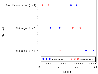
Nested two-factor ANOVA for the Training School data, table 28.4a, p. 1130.

proc glm data=training;
  class A B;
  model score = A B(A);
run;
quit;

The GLM Procedure

Class Level Information

Class Levels Values
A 3 1 2 3
B 2 1 2

Number of observations 12
The GLM Procedure
Dependent Variable: score
Sum of
Source DF Squares Mean Square F Value Pr > F
Model 5 724.0000000 144.8000000 20.69 0.0010
Error 6 42.0000000 7.0000000
Corrected Total 11 766.0000000

R-Square Coeff Var Root MSE score Mean
0.945170 17.63834 2.645751 15.00000

Source DF Type I SS Mean Square F Value Pr > F
A 2 156.5000000 78.2500000 11.18 0.0095
B(A) 3 567.5000000 189.1666667 27.02 0.0007
Source DF Type III SS Mean Square F Value Pr > F
A 2 156.5000000 78.2500000 11.18 0.0095
B(A) 3 567.5000000 189.1666667 27.02 0.0007

Decomposition of SSB(A), table 28.4b, p. 1130.
Note: Due to the large amount of output the SSB(Ai) have been italicized to make it easier to recognize them.

proc glm data=training;
  by A;
  class B ;
  model score = B;
run;
quit;

School=1

The GLM Procedure

Class Level Information

Class Levels Values
B 2 1 2

Number of observations 4
School=1

The GLM Procedure
Dependent Variable: score
Sum of
Source DF Squares Mean Square F Value Pr > F
Model 1 210.2500000 210.2500000 33.64 0.0285
Error 2 12.5000000 6.2500000
Corrected Total 3 222.7500000

R-Square Coeff Var Root MSE score Mean
0.943883 12.65823 2.500000 19.75000

Source DF Type I SS Mean Square F Value Pr > F
B 1 210.2500000 210.2500000 33.64 0.0285
Source DF Type III SS Mean Square F Value Pr > F
B 1 210.2500000 210.2500000 33.64 0.0285
School=2

The GLM Procedure

Class Level Information

Class Levels Values
B 2 1 2

Number of observations 4
School=2

The GLM Procedure
Dependent Variable: score
Sum of
Source DF Squares Mean Square F Value Pr > F
Model 1 132.2500000 132.2500000 12.90 0.0695
Error 2 20.5000000 10.2500000
Corrected Total 3 152.7500000

R-Square Coeff Var Root MSE score Mean
0.865794 22.46710 3.201562 14.25000

Source DF Type I SS Mean Square F Value Pr > F
B 1 132.2500000 132.2500000 12.90 0.0695
Source DF Type III SS Mean Square F Value Pr > F
B 1 132.2500000 132.2500000 12.90 0.0695
School=3

The GLM Procedure

Class Level Information

Class Levels Values
B 2 1 2

Number of observations 4
School=3

The GLM Procedure
Dependent Variable: score
Sum of
Source DF Squares Mean Square F Value Pr > F
Model 1 225.0000000 225.0000000 50.00 0.0194
Error 2 9.0000000 4.5000000
Corrected Total 3 234.0000000

R-Square Coeff Var Root MSE score Mean
0.961538 19.28473 2.121320 11.00000

Source DF Type I SS Mean Square F Value Pr > F
B 1 225.0000000 225.0000000 50.00 0.0194
Source DF Type III SS Mean Square F Value Pr > F
B 1 225.0000000 225.0000000 50.00 0.0194

Testing for factor B differences within level of factor A, specifically testing for
instructor differences within the Atlanta School, comments bottom of p. 1132.

ods listing close;
ods output  GLM.ANOVA.score.OverallANOVA=anova;
proc glm data=training;
  class A B;
  model score = A B(A);
run;
quit;
ods output GLM.ByGroup1.ANOVA.score.OverallANOVA=anova1;
proc glm data=training;
  by A;
  class B ;
  model score = B;
run;
quit;
ods listing;
ods output close;
data _null_;
  set anova;
  if source='Error' then call symput('mse', ms);
  if source='Error' then call symput('dfe', df);
run;
%put here are the macros: &mse and &dfe;
data _null_;
  set anova1;
  if source='Model' then call symput('msb_a1', ms);
  if source='Model' then call symput('dfb_a1', df);
run;
%put here are the macros: &msb_a1 and &dfb_a1;
data temp;
  F = &msb_a1 / &mse ;
  Fcrit = finv( .95, &dfb_a1, &dfe);
  p_value = 1 - probf(F, &dfb_a1, &dfe);
run;
proc print data=temp;
run;

Obs F Fcrit p_value

1 30.0357 5.98738 .001542714

Examining the residual of the nested model for the Training School data, fig. 28.4a, p. 1134.

proc glm data=training noprint;
  class A B;
  model score = A B(A);
  output out=resids r=resid;
run;
quit;
data resids;
  set resids;
  if a=1 then resid1=resid;
  if a=2 then resid2=resid;
  if a=3 then resid3=resid;
run;
 
symbol1 c=blue v=dot h=.8;
symbol2 c=red v=circle h=.8;
symbol3 c=green v=star h=.8;
axis1 label=('Residuals');
axis2 value=('Atlanta' 'Chicago' 'San Francisco');
proc gplot data=resids;
  plot a*(resid1 resid2 resid3)/ overlay vaxis=axis2 haxis=axis1;
run;
quit;

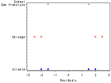
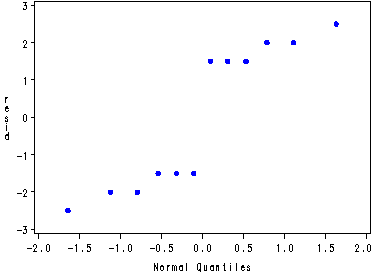
Normal probability plot of the residuals from the nested model, fig. 28.4b, p. 1134.

proc capability data=resids noprint;
   qqplot resid;
run;

Estimating the mean learning score for each school and calculating a 95% confidence coefficient
the mean learning score for the Atlanta school (a=1)with , p. 1135.

Note: The lsmean statement for B(A) gives the confidence interval using the Bonferroni coefficient for
all possible comparisons (6 choose 2 = 6!/2!4! = 30 )(B = t(1-.01/2*30, 6) = 7.31444) hence the
confidence intervals are much larger.

proc glm data=training;
  class a b;
  model score = a b(a);
  lsmeans A / cl adjust=tukey;
  lsmeans A / pdiff adjust=tukey cl alpha=.1;
  lsmeans B(A) / pdiff adjust=bon cl;
run;
quit;

The GLM Procedure

<output omitted>

Least Squares Means

A score LSMEAN

1 19.7500000
2 14.2500000
3 11.0000000

A score LSMEAN 95% Confidence Limits

1 19.750000 16.513040 22.986960
2 14.250000 11.013040 17.486960
3 11.000000 7.763040 14.236960

<output omitted>

Least Squares Means for effect A
Pr > |t| for H0: LSMean(i)=LSMean(j)

Dependent Variable: score

i/j 1 2 3
1 0.0586 0.0081
2 0.0586 0.2677
3 0.0081 0.2677

<output omitted>

Least Squares Means for Effect A

Difference Simultaneous 90%
Between Confidence Limits for
i j Means LSMean(i)-LSMean(j)
1 2 5.500000 0.792778 10.207222
1 3 8.750000 4.042778 13.457222
2 3 3.250000 -1.457222 7.957222

The GLM Procedure
Least Squares Means
Adjustment for Multiple Comparisons: Bonferroni

LSMEAN
B A score LSMEAN Number
1 1 27.0000000 1
2 1 12.5000000 2
1 2 8.5000000 3
2 2 20.0000000 4
1 3 18.5000000 5
2 3 3.5000000 6

<output omitted>

B A score LSMEAN 95% Confidence Limits

1 1 27.000000 22.422247 31.577753
2 1 12.500000 7.922247 17.077753
1 2 8.500000 3.922247 13.077753
2 2 20.000000 15.422247 24.577753
1 3 18.500000 13.922247 23.077753
2 3 3.500000 -1.077753 8.077753

Least Squares Means for Effect B(A)

Difference Simultaneous 95%
Between Confidence Limits for
i j Means LSMean(i)-LSMean(j)

1 2 14.500000 2.070465 26.929535
1 3 18.500000 6.070465 30.929535
1 4 7.000000 -5.429535 19.429535
1 5 8.500000 -3.929535 20.929535
1 6 23.500000 11.070465 35.929535
2 3 4.000000 -8.429535 16.429535
2 4 -7.500000 -19.929535 4.929535
2 5 -6.000000 -18.429535 6.429535

The GLM Procedure
Least Squares Means
Adjustment for Multiple Comparisons: Bonferroni

Least Squares Means for Effect B(A)

Difference Simultaneous 95%
Between Confidence Limits for
i j Means LSMean(i)-LSMean(j)

2 6 9.000000 -3.429535 21.429535
3 4 -11.500000 -23.929535 0.929535
3 5 -10.000000 -22.429535 2.429535
3 6 5.000000 -7.429535 17.429535
4 5 1.500000 -10.929535 13.929535
4 6 16.500000 4.070465 28.929535
5 6 15.000000 2.570465 27.429535

Testing three specific comparisons of treatment means: mu11-mu12, mu21-mu22, mu31-mu32, p. 1137.
It is a little tricky figuring out which difference of means correspond to the i and j columns in the last two
tables in the output above. The numbers for i and j refer to the list of the six lsmeans in the table
with the lsmean score before the two tables with confidence intervals in the above output. So, for the i=1, j=2
difference the second mean in the list (which is mu12) is begin subtracted from the first mean in the list (which is
mu11). Similarly, the i=3, j=4 difference is the fourth mean (mu22) being subtracted from the third mean (mu21).

ods listing close;
ods output GLM.LSMEANS.B_A_.score.LSMeanDiffCL=means  GLM.ANOVA.score.OverallANOVA=anova;
proc glm data=training;
  class a b;
  model score = a b(a);
  lsmeans B(A) / pdiff adjust=bon cl;
run;
quit;
ods listing;
ods output close;
data _null_;
  set anova;
  if source='Error' then call symput('mse', ms);
run;
%put here is the mse &mse; /* check number in SAS log file*/
data temp;
  set means;
  drop effect dependent LowerCL UpperCL;
  B = tinv(1 - (.01/2*3), 6);
  s2L = &mse*2/2; 
  BsL = B*sqrt(s2L);
  lower = difference - BsL;
  upper = difference + BsL;
run;
proc print data=temp;
  where (i=1 and j=2) or (i=3 and j=4) or (i=5 and j=6); 
  var difference B s2L BsL lower upper;
run;

Obs Difference B s2L BsL lower upper

1 14.500000 2.82893 7 7.48464 7.0154 21.9846
10 -11.500000 2.82893 7 7.48464 -18.9846 -4.0154
15 15.000000 2.82893 7 7.48464 7.5154 22.4846

Estimating the overall mean with a 95% confidence interval, p. 1137.

ods listing close;
ods output  OverallANOVA=anova  FitStatistics=fit;
proc glm data=training;
  class a b;
  model score = a b(a);
run;
quit;
ods output close;
ods listing;
data _null_;
  set anova;
  if source='Error' then call symput('mse', ms);
  if source='Error' then call symput('dfe', df);
  if source='Corrected Total' then call symput('df', df);
run;
%put here are the macros &mse &dfe &df; /*Check number in SAS log file*/
data _null_;
  set fit;
  call symput('mean', Depmean);
run;
%put here is the mean &mean; /*Check number in SAS log file*/
data temp;
  mean = &mean;
  s2Y = &mse/(&df+1);
  sY = sqrt(s2Y);
  t = tinv(.975, &dfe);
  lower = mean-t*sY;
  upper = mean + t*sY;
run;
proc print data=temp;
run;

Obs mean s2Y sY t lower upper

1 15 0.58333 0.76376 2.44691 13.1311 16.8689

Inputting Follow-up Training School study, table 28.6a, p. 1139.

data followup;
  input score A B rep;
  label A='School' 
        B='Instructor';
cards;
  20  1  1  1
  22  1  1  2
   8  1  2  1
   9  1  3  1
  13  1  3  2
   4  2  1  1
   8  2  1  2
  16  2  2  1
  20  2  2  2
;
run;

Generating the X and Y variables to be used in the regression, table 28.4b, p. 1139.

data reg;
  set followup;
  x1=1;
  if A=2 then x1=-1;
  x2=0;
  if A=1 and B=1 then x2=1;
  else if A=1 and B=3 then x2=-1;
  x3=0;
  if A=1 and B=2 then x3=1;
  else if A=1 and B=3 then x3=-1;
  x4=0;
  if A=2 and B=1 then x4=1;
  if A=2 and B=2 then x4=-1;
run;

The output from the tests statements correspond to the MS and Ftest statistics in table 28.7, p. 1141.

proc reg data=reg;
  model score = x1-x4;
  main_A: test x1=0;
  instructor_effect: test x2=x3=x4=0;
run;
quit;

The REG Procedure
Model: MODEL1
Dependent Variable: score

Analysis of Variance

Sum of Mean
Source DF Squares Square F Value Pr > F
Model 4 308.00000 77.00000 11.85 0.0172
Error 4 26.00000 6.50000
Corrected Total 8 334.00000

Root MSE 2.54951 R-Square 0.9222
Dependent Mean 13.33333 Adj R-Sq 0.8443
Coeff Var 19.12132

Parameter Estimates

Parameter Standard
Variable DF Estimate Error t Value Pr > |t|
Intercept 1 12.66667 0.87599 14.46 0.0001
x1 1 0.66667 0.87599 0.76 0.4890
x2 1 7.66667 1.58990 4.82 0.0085
x3 1 -5.33333 1.90029 -2.81 0.0485
x4 1 -6.00000 1.27475 -4.71 0.0093

The REG Procedure
Model: MODEL1

Test main_A Results for Dependent Variable score

Mean
Source DF Square F Value Pr > F
Numerator 1 3.76471 0.58 0.4890
Denominator 4 6.50000

The REG Procedure
Model: MODEL1

Test instructor_effect Results
for Dependent Variable score

Mean
Source DF Square F Value Pr > F
Numerator 3 98.40000 15.14 0.0119
Denominator 4 6.50000

You can obtain the same results using proc glm and the option ss3 which is robust to unequal
sample sizes, table 28.7, p. 1141.

proc glm data=followup;
  class a b;
  model score= a b(a) / ss3;
run;
quit;

The GLM Procedure

Class Level Information

Class Levels Values
A 2 1 2
B 3 1 2 3

Number of observations 9
The GLM Procedure
Dependent Variable: score
Sum of
Source DF Squares Mean Square F Value Pr > F
Model 4 308.0000000 77.0000000 11.85 0.0172
Error 4 26.0000000 6.5000000
Corrected Total 8 334.0000000

R-Square Coeff Var Root MSE score Mean
0.922156 19.12132 2.549510 13.33333

Source DF Type III SS Mean Square F Value Pr > F
A 1 3.7647059 3.7647059 0.58 0.4890
B(A) 3 295.2000000 98.4000000 15.14 0.0119

Inputting the Bread Crustiness data, table 28.9, p. 1144.

data bread;
  input score a b rep;
  label a ='Temperature'
        b ='Batch'
      rep ='Exp. unit';
cards;
   4  1  1  1
   7  1  1  2
   5  1  1  3
  12  1  2  1
   8  1  2  2
  10  1  2  3
  14  2  1  1
  13  2  1  2
  11  2  1  3
   9  2  2  1
  10  2  2  2
  12  2  2  3
  14  3  1  1
  17  3  1  2
  15  3  1  3
  16  3  2  1
  19  3  2  2
  18  3  2  3
;
run;

Fig. 28.5, p. 1144.

data plot;
  set bread;
  if b=1 then b1=score;
  if b=2 then b2=score;
run;
goptions reset=all;

symbol1 c=blue v=dot;
symbol2 c=red v=circle;
axis1 value=('Low (i=1)' 'Medium (i=2)' 'High (i=3)' ) offset=(2,5);
axis2 label=('Crustiness') order=(0 to 20 by 5);
legend1 label=none value=(height=.8 font=swiss 'Batch=1' 'Batch=2' ) 
        position=(top left inside) mode=share cborder=black;
proc gplot data=plot;
  plot a*(b1 b2)/ overlay vaxis=axis1 haxis=axis2 legend=legend1;
run;
quit;

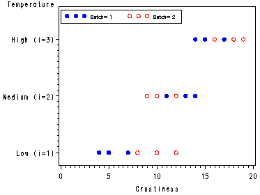
ANOVA table 28.10, and tests of temperature effect and batch differences, p. 1144-1145. Estimating
treatment effects, including the mean of the low temperature group and the difference between the low and high
temperature groups with a 95% confidence interval, p. 1146.

proc glm data=bread;
  class a b;
  model score = a b(a);
  random b(a);
  temperature_effect: test h=a e=b(a);
  lsmeans a / e=b(a) pdiff cl;
run;
quit;

The GLM Procedure

Class Level Information

Class Levels Values
a 3 1 2 3
b 2 1 2

Number of observations 18
The GLM Procedure
Dependent Variable: score
Sum of
Source DF Squares Mean Square F Value Pr > F
Model 5 284.4444444 56.8888889 21.79 <.0001
Error 12 31.3333333 2.6111111
Corrected Total 17 315.7777778

R-Square Coeff Var Root MSE score Mean
0.900774 13.59163 1.615893 11.88889

Source DF Type I SS Mean Square F Value Pr > F
a 2 235.4444444 117.7222222 45.09 <.0001
b(a) 3 49.0000000 16.3333333 6.26 0.0084
Source DF Type III SS Mean Square F Value Pr > F
a 2 235.4444444 117.7222222 45.09 <.0001
b(a) 3 49.0000000 16.3333333 6.26 0.0084

The GLM Procedure

Source Type III Expected Mean Square
a Var(Error) + 3 Var(b(a)) + Q(a)
b(a) Var(Error) + 3 Var(b(a))

The GLM Procedure
Least Squares Means
Standard Errors and Probabilities Calculated Using the Type III MS for b(a) as an Error Term

LSMEAN
a score LSMEAN Number
1 7.6666667 1
2 11.5000000 2
3 16.5000000 3

Least Squares Means for effect a
Pr > |t| for H0: LSMean(i)=LSMean(j)

Dependent Variable: score

i/j 1 2 3
1 0.1990 0.0323
2 0.1990 0.1215
3 0.0323 0.1215

a score LSMEAN 95% Confidence Limits
1 7.666667 2.415898 12.917435
2 11.500000 6.249231 16.750769
3 16.500000 11.249231 21.750769

Least Squares Means for Effect a

Difference
Between 95% Confidence Limits for
i j Means LSMean(i)-LSMean(j)
1 2 -3.833333 -11.259041 3.592375
1 3 -8.833333 -16.259041 -1.407625
2 3 -5.000000 -12.425708 2.425708

NOTE: To ensure overall protection level, only probabilities associated with pre-planned
comparisons should be used.

The GLM Procedure

Dependent Variable: score

Tests of Hypotheses Using the Type III MS for b(a) as an Error Term

Source DF Type III SS Mean Square F Value Pr > F
a 2 235.4444444 117.7222222 7.21 0.0715

Tests of the main effects of temperature, p. 1144-1145. Estimating treatment effects, including
the mean of the low temperature group and the difference between the low and high temperature groups with a
95% confidence intervals using proc mixed, p. 1146.

proc mixed data=bread;
  class a b;
  model score = a;
  random b(a);
  lsmeans a / cl pdiff;
run;
quit;

The Mixed Procedure

Model Information
Data Set WORK.BREAD
Dependent Variable score
Covariance Structure Variance Components
Estimation Method REML
Residual Variance Method Profile
Fixed Effects SE Method Model-Based
Degrees of Freedom Method Containment

Class Level Information

Class Levels Values
a 3 1 2 3
b 2 1 2

Dimensions
Covariance Parameters 2
Columns in X 4
Columns in Z 6
Subjects 1
Max Obs Per Subject 18
Observations Used 18
Observations Not Used 0
Total Observations 18

Iteration History

Iteration Evaluations -2 Res Log Like Criterion
0 1 73.11545106
1 1 67.84036856 0.00000000

Convergence criteria met.
Covariance Parameter
Estimates

Cov Parm Estimate
b(a) 4.5741
Residual 2.6111

The Mixed Procedure

Fit Statistics
-2 Res Log Likelihood 67.8
AIC (smaller is better) 71.8
AICC (smaller is better) 72.8
BIC (smaller is better) 71.4

Type 3 Tests of Fixed Effects

Num Den
Effect DF DF F Value Pr > F
a 2 3 7.21 0.0715

Least Squares Means

Standard
Effect Temperature Estimate Error DF t Value Pr > |t| Alpha Lower Upper
a 1 7.6667 1.6499 3 4.65 0.0188 0.05 2.4159 12.9174
a 2 11.5000 1.6499 3 6.97 0.0061 0.05 6.2492 16.7508
a 3 16.5000 1.6499 3 10.00 0.0021 0.05 11.2492 21.7508

Differences of Least Squares Means

Standard
Effect Temperature Temperature Estimate Error DF t Value Pr > |t| Alpha
a 1 2 -3.8333 2.3333 3 -1.64 0.1990 0.05
a 1 3 -8.8333 2.3333 3 -3.79 0.0323 0.05
a 2 3 -5.0000 2.3333 3 -2.14 0.1215 0.05

Differences of Least Squares Means

Effect Temperature Temperature Lower Upper
a 1 2 -11.2590 3.5924
a 1 3 -16.2590 -1.4076
a 2 3 -12.4257 2.4257

Unable to reproduce the same results as in the book for the estimation of sigma-squared
(between batch variability), p. 1146-1147.

Inputting the Group Decision Making data, table 28.12, p. 1152.

data decision;
  input score a b c rep ;
  label a ='Nationality'
        b ='Size'
	c ='Observer';
cards;
  16  1  1  1  1
  20  1  1  1  2
  14  1  1  2  1
  19  1  1  2  2
   7  2  1  1  1
   5  2  1  1  2
   4  2  1  2  1
   9  2  1  2  2
  21  1  2  1  1
  25  1  2  1  2
  28  1  2  2  1
  19  1  2  2  2
  11  2  2  1  1
  17  2  2  1  2
  12  2  2  2  1
  15  2  2  2  2
;
run;

Fig. 28.6, p. 1152.

data plot;
  set decision;
  if a=1 and c=1 then a1c1=score;
  if a=1 and c=2 then a1c2=score;
  if a=2 and c=1 then a2c1=score;
  if a=2 and c=2 then a2c2=score;
run;
goptions reset=all;
 
symbol1 c=red v=square;
symbol2 c=green v=circle;
symbol3 c=blue v=:;
symbol4 c=cyan v=dot;
axis1 label=(a=90 'Size of Team') value=('4' '8') offset=(10,5) order=(1 2);
axis2 label=('Number of Group Interactions');
legend1 label=none value=(height=.8 font=swiss 'US, observer 1' 'US, observer 2' 
        'Foreign, observer 1' 'Foreign, observer 2' ) across=2 
        position=(bottom right inside) mode=share cborder=black;
proc gplot data=plot;
  plot b*(a1c1 a1c2 a2c1 a2c2) / overlay vaxis=axis1 haxis=axis2 legend=legend1; 
run;
quit;

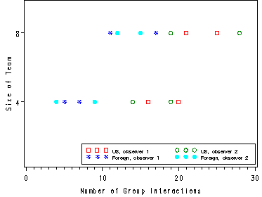
Fig. 28.7, p. 1153 and estimating the difference in mean score between US and Foreign teams, p. 1154.

proc glm data=decision;
  class a b c;
  model score = A | c(A) | b;
  test h=a e=c(a);
  lsmeans a / e=c(a) cl pdiff;
run;
quit;

The GLM Procedure

Class Level Information

Class Levels Values
a 2 1 2
b 2 1 2
c 2 1 2

Number of observations 16
The GLM Procedure
Dependent Variable: score

Sum of
Source DF Squares Mean Square F Value Pr > F
Model 7 607.7500000 86.8214286 6.55 0.0083
Error 8 106.0000000 13.2500000
Corrected Total 15 713.7500000

R-Square Coeff Var Root MSE score Mean
0.851489 24.06648 3.640055 15.12500

Source DF Type I SS Mean Square F Value Pr > F
a 1 420.2500000 420.2500000 31.72 0.0005
c(a) 2 0.5000000 0.2500000 0.02 0.9814
b 1 182.2500000 182.2500000 13.75 0.0060
a*b 1 2.2500000 2.2500000 0.17 0.6911
b*c(a) 2 2.5000000 1.2500000 0.09 0.9110

Source DF Type III SS Mean Square F Value Pr > F
a 1 420.2500000 420.2500000 31.72 0.0005
c(a) 2 0.5000000 0.2500000 0.02 0.9814
b 1 182.2500000 182.2500000 13.75 0.0060
a*b 1 2.2500000 2.2500000 0.17 0.6911
b*c(a) 2 2.5000000 1.2500000 0.09 0.9110

Tests of Hypotheses Using the Type III MS for c(a) as an Error Term

Source DF Type III SS Mean Square F Value Pr > F
a 1 420.2500000 420.2500000 1681.00 0.0006

The GLM Procedure
Least Squares Means
Standard Errors and Probabilities Calculated Using the Type III MS for c(a) as an Error Term

H0:LSMean1=
LSMean2
a score LSMEAN Pr > |t|
1 20.2500000 0.0006
2 10.0000000
a score LSMEAN 95% Confidence Limits
1 20.250000 19.489391 21.010609
2 10.000000 9.239391 10.760609

Least Squares Means for Effect a

Difference
Between 95% Confidence Limits for
i j Means LSMean(i)-LSMean(j)
1 2 10.250000 9.174337 11.325663