Applied Linear Statistical Models by Neter, Kutner, et. al. Chapter 3: Diagnostics and Remedial Measures | SAS Textbook Examples

Inputting the Toluca Company data.

data ch1tab01;
  input x y;
  label x = 'Lot Size'
        y = 'Work Hrs';
cards;
   80  399
   30  121
   50  221
   90  376
   70  361
   60  224
  120  546
   80  352
  100  353
   50  157
   40  160
   70  252
   90  389
   20  113
  110  435
  100  420
   30  212
   50  268
   90  377
  110  421
   30  273
   90  468
   40  244
   80  342
   70  323
;
run;

Fig. 3.1a,c and d, p. 96.

proc univariate plots data = ch1tab01;
 var x;
run;

The UNIVARIATE Procedure

Variable:  x  (Lot Size)

                            Moments

N                          25    Sum Weights                 25

Mean                       70    Sum Observations          1750

Std Deviation      28.7228132    Variance                   825

Skewness           -0.1032081    Kurtosis            -1.0794107

Uncorrected SS         142300    Corrected SS             19800

Coeff Variation    41.0325903    Std Error Mean      5.74456265
              Basic Statistical Measures
    Location                    Variability
Mean     70.00000     Std Deviation           28.72281

Median   70.00000     Variance               825.00000

Mode     90.00000     Range                  100.00000

                      Interquartile Range     40.00000
           Tests for Location: Mu0=0
Test           -Statistic-    —–p Value——
Student’s t    t  12.18544    Pr > |t|    <.0001

Sign           M      12.5    Pr >= |M|   <.0001

Signed Rank    S     162.5    Pr >= |S|   <.0001
Quantiles (Definition 5)
Quantile      Estimate
100% Max           120

99%                120

95%                110

90%                110

75% Q3              90

50% Median          70

25% Q1              50

10%                 30

5%                  30

1%                  20

0% Min              20
The UNIVARIATE Procedure

Variable:  x  (Lot Size)
        Extreme Observations
—-Lowest—-        —-Highest—
Value      Obs        Value      Obs
   20       14          100        9

   30       21          100       16

   30       17          110       15

   30        2          110       20

   40       23          120        7
   Stem Leaf                     #  Boxplot

     12 0                        1     |

     11 00                       2     |

     10 00                       2     |

      9 0000                     4  +—–+

      8 000                      3  |     |

      7 000                      3  *–+–*

      6 0                        1  |     |

      5 000                      3  +—–+

      4 00                       2     |

      3 000                      3     |

      2 0                        1     |

        —-+—-+—-+—-+

    Multiply Stem.Leaf by 10**+1
                       Normal Probability Plot

     125+                                           ++*

        |                                      *+*++

        |                                  * *++

        |                             ***+*++

        |                          ***+++

      75+                       ***+++

        |                      *++

        |                   ***

        |               +**+

        |          * *+*

      25+     *  ++++

         +—-+—-+—-+—-+—-+—-+—-+—-+—-+—-+

             -2        -1         0        +1        +2

Fig. 3.1b, p. 96.

data temp;
  set ch1tab01;
  id = _n_;
  group=1;
run;
 
goptions reset = all;
symbol1 v=dot h=.8 i=join;
proc gplot data = temp;
  plot x*id;
run;
quit;

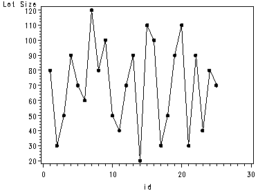
Fig. 3.2a and 3.2d, p. 99.

symbol1 v=dot h=.8 c=blue;
proc reg data = temp noprint;
  model y = x;
  output out=temp1 r=r;
  plot r.*x r.*nqq.;
run;
quit;
symbol1 v=dot h=.8 c=blue i=none;
proc boxplot data=temp1 ;
  plot r*group;
run;

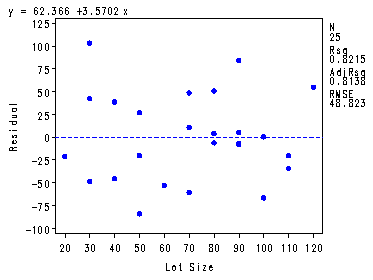
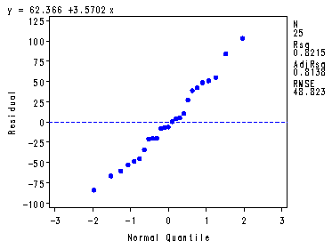
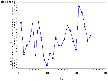
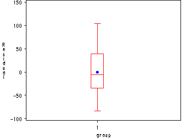
Fig. 3.2b and c, p. 99.

symbol1 v=dot h=.8 c= blue i=join;
proc gplot data = temp1;
  plot r*id;
run;
quit;
symbol1 v=dot h=.8 c=blue i=none;
proc boxplot data=temp1 ;
  plot r*group;
run;

Inputting the Transit data, p. 100.

data ch3tab01;
  input y x;
  label y = 'Ridership'
        x = 'Maps';
cards;
   .60   80
  6.70  220
  5.30  140
  4.00  120
  6.55  180
  2.15  100
  6.60  200
  5.75  160
;
run;

Fig. 3.3, p. 100.

proc reg data = ch3tab01 noprint;
  model y = x;
  plot y*x r.*x r.*nqq.;
  output out=temp r=residual p=yhat;
run;
quit;

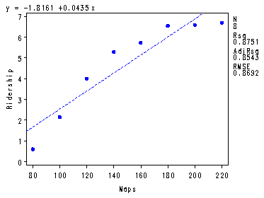
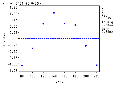
Table 3.1, p. 100.

proc reg data = ch3tab01 noprint;
  model y = x;
  output out = temp p=yhat r=residual;
run;
proc print data = temp;
  var y x yhat residual;
run;

Obs      y      x       yhat     residual

 1     0.60     80    1.66250    -1.06250

 2     6.70    220    7.75000    -1.05000

 3     5.30    140    4.27143     1.02857

 4     4.00    120    3.40179     0.59821

 5     6.55    180    6.01071     0.53929

 6     2.15    100    2.53214    -0.38214

 7     6.60    200    6.88036    -0.28036

 8     5.75    160    5.14107     0.60893

Table 3.2, p. 106.

data temp;
  set ch1tab01;
  id = _n_;
run;
proc reg data = temp noprint;
  model y = x;
  output out=temp1 r=r;
run;
quit;
proc sort data = temp1;
  by r;
run;
data temp2 ;
  set temp1;
  k = _n_;
run;
proc rank data = temp2 normal = blom out=temp3 ;
  var r;
  ranks k1;
run;
data temp3;
  set temp3;
  expected = k1*sqrt(2384);
run;
proc sort data = temp3;
  by id;
run;
proc print data = temp3;
  var id r k expected;
run;

Obs    id           r     k    expected

  1     1      51.018    22     51.9727

  2     2     -48.472     5    -44.1075

  3     3     -19.876    10    -14.7632

  4     4      -7.684    11     -9.7588

  5     5      48.720    21     44.1075

  6     6     -52.578     4    -51.9727

  7     7      55.210    23     61.4870

  8     8       4.018    15      9.7588

  9     9     -66.386     2    -74.1767

 10    10     -83.876     1    -95.9053

 11    11     -45.174     6    -37.2478

 12    12     -60.280     3    -61.4870

 13    13       5.316    16     14.7632

 14    14     -20.770     8    -25.3268

 15    15     -20.088     9    -19.9281

 16    16       0.614    14      4.8551

 17    17      42.528    20     37.2478

 18    18      27.124    18     25.3268

 19    19      -6.684    12     -4.8551

 20    20     -34.088     7    -31.0553

 21    21     103.528    25     95.9053

 22    22      84.316    24     74.1767

 23    23      38.826    19     31.0553

 24    24      -5.982    13     -0.0000

 25    25      10.720    17     19.9281

The Modified Levene test of constancy of error variance, p. 112-114 and Table 3.3,
p. 114.  The values of mr in the output correspond to the mean of
the residuals for each group and the values of md correspond to mean of the
deviations for each group. 
Note1: The two-sample t-test corresponds to the pooled variance t-test
in the proc ttest output.

Note2: SAS does have a Levene test option in proc GLM but it is not the same as the modified
Levene test described in this section.

proc reg data = ch1tab01 noprint;
  model y = x;
  output out=temp r=r;
run;
data temp1;
  set temp;
  id = _n_;
  group = .;
  if x <= 70 then group = 1;
  if x > 70 then group = 2;
run;
proc sort data = temp1;
  by group;
run;
proc means data = temp1 noprint;
  by group;
  var r;
  output out=mout median=mr;
run;
proc print data = mout;
 var group mr;
run;
data mtemp;
  merge temp1 mout;
  by group;
  d = abs(r - mr);
run;
proc sort data = mtemp;
  by group;
run; 
proc means data = mtemp noprint;
  by group;
  var d;
  output out=mout1 mean=md;
run;
proc print data = mout1;
  var group md;
run;
data mtemp1;
  merge mtemp mout1;
  by group;
  ddif = (d - md)**2;
run;
proc sort data = mtemp1;
 by group x;
run;
proc ttest data = mtemp1;
  class group;
  var d;
run;
proc print data = mtemp1; 
 by group;
 var id x r d ddif;
run;

Obs    group       mr

 1       1      -19.8760

 2       2       -2.6840

Obs    group       md
 1       1      44.8151

 2       2      28.4503
The TTEST Procedure
                                           Statistics
                              Lower CL          Upper CL  Lower CL           Upper CL

Variable  group            N      Mean    Mean      Mean   Std Dev  Std Dev   Std Dev  Std Err

d                         13     25.26  44.815     64.37    23.205   32.361    53.419   8.9753

          1

d                         12    9.6702   28.45     47.23    20.939   29.558    50.186   8.5326

          2

d         Diff (1-2)             -9.35  16.365     42.08    24.134   31.052    43.558   12.431
                               T-Tests
Variable    Method           Variances      DF    t Value    Pr > |t|

d           Pooled           Equal          23       1.32      0.2010

d           Satterthwaite    Unequal        23       1.32      0.1993
                    Equality of Variances
Variable    Method      Num DF    Den DF    F Value    Pr > F

d           Folded F        12        11       1.20    0.7710

group=1
Obs    id     x        r             d       ddif
  1    14    20     -20.770      0.894    1929.07

  2     2    30     -48.472     28.596     263.06

  3    17    30      42.528     62.404     309.37

  4    21    30     103.528    123.404    6176.23

  5    11    40     -45.174     25.298     380.92

  6    23    40      38.826     58.702     192.85

  7     3    50     -19.876      0.000    2008.39

  8    10    50     -83.876     64.000     368.06

  9    18    50      27.124     47.000       4.77

 10     6    60     -52.578     32.702     146.73

 11     5    70      48.720     68.596     565.53

 12    12    70     -60.280     40.404      19.46

 13    25    70      10.720     30.596     202.18
group=2

Obs    id     x            r       d          ddif
 14     1     80     51.0180    53.7020     637.65

 15     8     80      4.0180     6.7020     472.99

 16    24     80     -5.9820     3.2980     632.64

 17     4     90     -7.6840     5.0000     549.92

 18    13     90      5.3160     8.0000     418.22

 19    19     90     -6.6840     4.0000     597.82

 20    22     90     84.3160    87.0000    3428.06

 21     9    100    -66.3861    63.7020    1242.68

 22    16    100      0.6139     3.2980     632.64

 23    15    110    -20.0881    17.4040     122.02

 24    20    110    -34.0881    31.4040       8.72

 25     7    120     55.2099    57.8939     866.93

The Breusch-Pagan test, p. 115.

Note1: SAS has a modified Breusch-Pagan test as an
option in the model procedure but it is not exactly the same test as in the book. As for the
test in the book, SAS can provide the components of the test statistic separately and
it is possible to perform the test manually.
Note2: The book reports the p-value for this test as .64.  We believe
that the correct p-value for this test should be .36 = (1-.64) as reported.

ods listing close;
proc reg data = ch1tab01;
  model y = x;
  ods output ANOVA = temp1;
  output out= temp r=e;
run;
quit;
ods listing;
data temp1;
  set temp1;
  if source='Error' then call symput ('sse' , ss);
run;
data temp2;
  set temp nobs=total;
  e2 = e**2;
run;
ods listing close;
proc reg data = temp2;
  model e2 = x;
  ods output anova = temp3;
run;
quit;
ods listing;
data temp3;
  set temp3;
  if source='Model' then call symput ('ssr', ss);
run;
data tempf;
  set tempf;
  pvalue = 1-probchi( (&ssr/2)/(&sse/25)**2 , 1 );
  ssr = &ssr;
  sse = &sse;
run;
proc print data= tempf ;
 var ssr sse pvalue;
run;

Obs            ssr            sse        pvalue	

 1         7896142          54825        .3649

The modified Breusch-Pagan Test as an option in the model procedure. For more explanation
of this test please refer to the SAS Manual under heteroscedasticity.

proc model data=ch1tab01;
  parms const beta ;
  y = const + beta * x ;
  fit y / white breusch=(1 x);
run;
quit;

The MODEL Procedure

      Model Summary

Model Variables         1

Parameters              2

Equations               1

Number of Statements    1
Model Variables  y

     Parameters  const beta

      Equations  y
The Equation to Estimate is

y =  F(const(1), beta(x))
NOTE: At OLS Iteration 1 CONVERGE=0.001 Criteria Met.
The MODEL Procedure

OLS Estimation Summary
Data Set Options

DATA=    CH1TAB01

      Minimization Summary

Parameters Estimated            2

Method                      Gauss

Iterations                      1
Final Convergence Criteria

R                         0

PPC                       0

RPC(const)         617482.8

Object             0.980028

Trace(S)           2383.716

Objective Value    2193.018
Observations Processed

Read      25

Solved    25
The MODEL Procedure
                    Nonlinear OLS Summary of Residual Errors
                   DF       DF                                            Adj

Equation        Model    Error         SSE         MSE    R-Square       R-Sq

y                   2       23     54825.5      2383.7      0.8215     0.8138
             Nonlinear OLS Parameter Estimates
                              Approx                  Approx

Parameter       Estimate     Std Err    t Value     Pr > |t|

const           62.36586     26.1774       2.38       0.0259

beta            3.570202      0.3470      10.29       <.0001
Number of Observations     Statistics for System

Used                25    Objective           2193

Missing              0    Objective*N        54825

                                 Heteroscedasticity Test

Equation        Test               Statistic     DF    Pr > ChiSq    Variables

y               White’s Test            1.33      2        0.5142    Cross of all vars

                Breusch-Pagan           1.13      1        0.2872    1, x

Inputting the Bank data, Table 3.4, p. 117.

data ch3tab04;
  input x y;
  label x = 'deposit'
        y = 'new accounts';
cards;
  125  160
  100  112
  200  124
   75   28
  150  152
  175  156
   75   42
  175  124
  125  150
  200  104
  100  136
;
run;

Table 3.4b, The Anova table, p. 117.

proc reg data =ch3tab04;
  model y = x;
run;
quit;

The REG Procedure

Model: MODEL1

Dependent Variable: y new accounts

                             Analysis of Variance
                                    Sum of           Mean

Source                   DF        Squares         Square    F Value    Pr > F

Model                     1     5141.33841     5141.33841       3.14    0.1102

Error                     9          14742     1637.95230

Corrected Total          10          19883
Root MSE             40.47162    R-Square     0.2586

Dependent Mean      117.09091    Adj R-Sq     0.1762

Coeff Var            34.56427
                                Parameter Estimates
                                     Parameter       Standard

Variable     Label           DF       Estimate          Error    t Value    Pr > |t|

Intercept    Intercept        1       50.72251       39.39791       1.29      0.2301

x            deposit          1        0.48670        0.27471       1.77      0.1102

Using proc transpose to create table 3.5, data arranged by replicates of X, p. 117.

proc sort data = ch3tab04;
by x;
proc transpose data = ch3tab04 out=wide;
 by x;
run;
proc print data = wide (rename = (col1 = rep1 col2 = rep2) );
  var x rep1 rep2;
run;

Obs     x     rep1    rep2

 1      75      28      42

 2     100     112     136

 3     125     160     150

 4     150     152       .

 5     175     156     124

 6     200     124     104

Getting the means of Y per value of X, the last line in table 3.5, p. 117.

proc means data = ch3tab04 mean;
  by x;
  var y;
run;

deposit=75

The MEANS Procedure
Analysis Variable : y new accounts
        Mean

————

  35.0000000

————

deposit=100
Analysis Variable : y new accounts
        Mean

————

 124.0000000

————

deposit=125
Analysis Variable : y new accounts
        Mean

————

 155.0000000

————

deposit=150
Analysis Variable : y new accounts
        Mean

————

 152.0000000

————

deposit=175
The MEANS Procedure
Analysis Variable : y new accounts
        Mean

————

 140.0000000

————

deposit=200
Analysis Variable : y new accounts
        Mean

————

 114.0000000

————

Table 3.6b, p. 123. The f variable in output is the test statistic used in the test for lack of fit.

proc reg data = ch3tab04;
  model y = x;
  output out=temp p=p;
run;
proc sql;
  create table temp1 as
  select *, (y - mean(y))**2 as sspe1, (mean(y) - p)**2 as sslf1
  from temp
  group by x;
quit;
proc sql;
  create table temp2 as
  select *, sum( sspe1 ) as sspe, sum( sslf1 ) as sslf
  from temp1;
quit;
proc sort data = temp2;
  by sspe sslf;
run; 
data temp3 (keep = sspe sslf f pvalue);
  set temp2;
  by sspe sslf;
  if first.sspe;
  f = (sslf/4) / (sspe/5);
  pvalue = 1 - probf( f, 4, 5);
run;
proc print data = temp3;
run;

The REG Procedure

Model: MODEL1

Dependent Variable: y new accounts

                             Analysis of Variance
                                    Sum of           Mean

Source                   DF        Squares         Square    F Value    Pr > F

Model                     1     5141.33841     5141.33841       3.14    0.1102

Error                     9          14742     1637.95230

Corrected Total          10          19883
Root MSE             40.47162    R-Square     0.2586

Dependent Mean      117.09091    Adj R-Sq     0.1762

Coeff Var            34.56427
                                Parameter Estimates
                                     Parameter       Standard

Variable     Label           DF       Estimate          Error    t Value    Pr > |t|

Intercept    Intercept        1       50.72251       39.39791       1.29      0.2301

x            deposit          1        0.48670        0.27471       1.77      0.1102

Obs    sspe      sslf         f           pvalue
 1     1148    13593.57    14.8014    .005593812

Inputting Sales Training data, table 3.7, p. 127.

data ch3tab07;
  input x y;
  label x = 'Training'
        y = 'Performance';
cards;
  0.5   42.5
  0.5   50.6
  1.0   68.5
  1.0   80.7
  1.5   89.0
  1.5   99.6
  2.0  105.3
  2.0  111.8
  2.5  112.3
  2.5  125.7
;
run;

Transforming X as sqrt(X).

data ch3tab07;
  set ch3tab07;
  sqrtX = sqrt(x);
run;

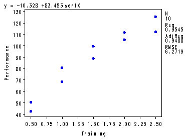
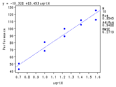
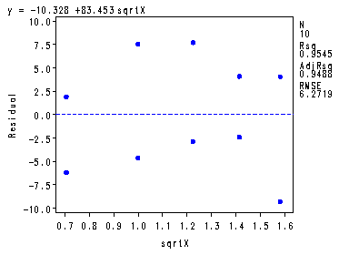
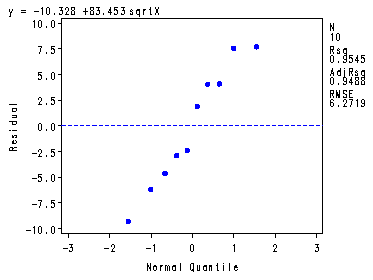
Fig. 3.14 and the fitted regression function at the bottom of p. 128.

symbol1 v=dot c=blue h=.8;
proc reg data = ch3tab07;
  var x;
  model y = sqrtx;
  plot y*x y*sqrtx r.*sqrtx r.*nqq.;
run;
quit;

Inputting Plasma Levels data, table 3.8, p. 130.

data ch3tab08;
  input x y logy;
  label x = 'Age'
        y = 'Plasma'
     logy = 'Log(plasma)';
cards;
    0  13.44  1.1284
    0  12.84  1.1086
    0  11.91  1.0759
    0  20.09  1.3030
    0  15.60  1.1931
  1.0  10.11  1.0048
  1.0  11.38  1.0561
  1.0  10.28  1.0120
  1.0   8.96   .9523
  1.0   8.59   .9340
  2.0   9.83   .9926
  2.0   9.00   .9542
  2.0   8.65   .9370
  2.0   7.85   .8949
  2.0   8.88   .9484
  3.0   7.94   .8998
  3.0   6.01   .7789
  3.0   5.14   .7110
  3.0   6.90   .8388
  3.0   6.77   .8306
  4.0   4.86   .6866
  4.0   5.10   .7076
  4.0   5.67   .7536
  4.0   5.75   .7597
  4.0   6.23   .7945
;
run;

Fitted regression function at the bottom of p. 129 and Fig. 3.16, p. 131.

symbol1 v=dot c=blue h =.8;
proc reg data = ch3tab08;
  var y;
  model logy = x;
  plot y*x logy*x r.*x r.*nqq.;
run;
quit;

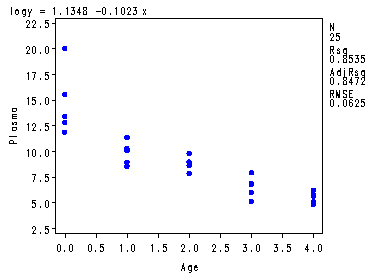
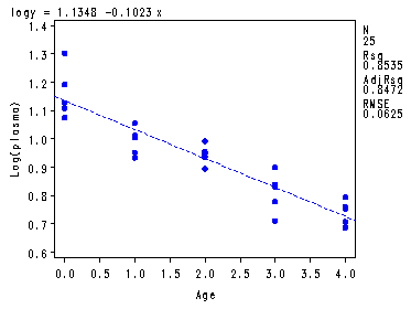
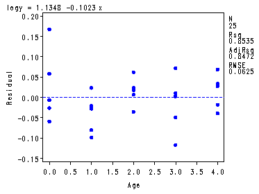
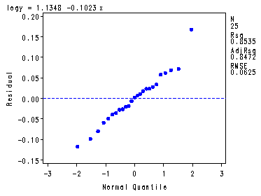
Table 3.9, p. 134. SAS does not automatically print out a table like this but there are
macros that will create very similar tables. In a search of the web we found a boxcox
macros and an explanation of how to use it at:
http://www.math.yorku.ca/SCS/sasmac/boxcox.html

%boxcox(resp=y, model= x, data = ch3tab08);

Fig. 3.18a, p. 138.

ods listing close;
proc loess data = ch1tab01 ;
  model y = x / degree=2  smooth = .85;
  ods output OutputStatistics=results;
run;
ods listing;
proc sort data = results;
 by x;
run;
 
goptions reset = all;
 
symbol1 v=none c=blue i=join ;
symbol2 v=dot c=blue i=none h=.8; 
axis1 order=(0 to 150 by 50);
proc gplot data=Results; 
 plot  DepVar*x=2 pred*x=1/overlay haxis=axis1;
run;
quit;
goptions reset=all;

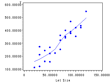
Fig. 3.18b, p. 138.

ods listing close;
proc loess data = ch1tab01 ;
  model y = x / degree=2  smooth = .85;
  ods output OutputStatistics=results;
run;
ods listing;
proc sort data = results;
 by x;
run;
data results1 (rename = ( Depvar=y pred=loess) );
  set results;
run;
proc reg data = results1 noprint;
 model y = x;
 output out=temp lclm=lower uclm=upper;
run;
quit;
 
symbol1 v=none i=join c=red line=20;
symbol2 v=none h=.4 i=join c=black;
symbol3 v=none i=join c=red line=20;
axis1 label=(angle=90 'hours');
axis2 order=(0 to 150 by 50);
proc gplot data = temp;
  plot (lower loess upper)*x/ overlay vaxis=axis1 haxis=axis2;
run;
quit;
goptions reset=all;

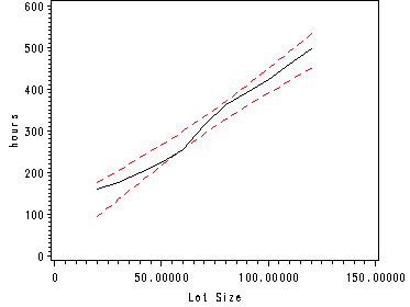
Inputting the Plutonium Measurement data, table 3.10, p. 139.

data ch3tab10;
  input y x ; 
  label x = 'Plutonium Activity, pCi/g'
        y = 'Alpha Count, #/sec.';
cards;
  0.150  20
  0.004   0
  0.069  10
  0.030   5
  0.011   0
  0.004   0
  0.041   5
  0.109  20
  0.068  10
  0.009   0
  0.009   0
  0.048  10
  0.006   0
  0.083  20
  0.037   5
  0.039   5
  0.132  20
  0.004   0
  0.006   0
  0.059  10
  0.051  10
  0.002   0
  0.049   5
  0.106   0
;
run;

Fig. 3.19a, p. 139.

symbol1 v=dot h=.8 c=blue;
proc gplot data=ch3tab10;
  plot y*x;
run;
quit;

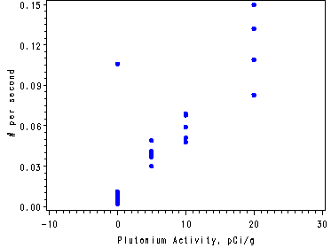
Fig. 3.19b, p. 139.

ods listing close;
proc loess data = ch3tab10 ;
  model y = x / degree=2  smooth = .85;
  ods output OutputStatistics=results;
run;
ods listing;
proc sort data = results;
 by x;
run;
 
axis1 order=(-10 to 30 by 10);
axis2 order=(0 to .15 by .03);
symbol1 v=none c=blue i=join;
symbol2 v=dot c=blue i=none; 
proc gplot data=Results; 
 plot  DepVar*x=2 pred*x=1/overlay haxis=axis1 vaxis=axis2;
run;
quit;
goptions reset=all;

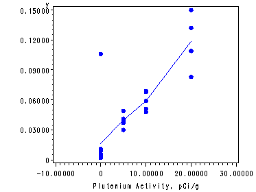
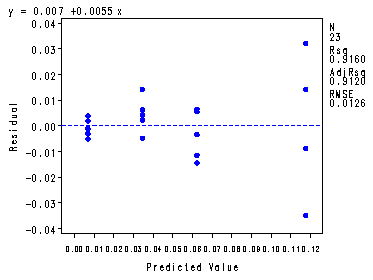
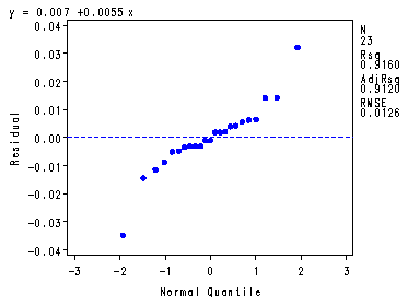
Fig. 3.20, p. 140.

Note: The where statement eliminates observation #24.

symbol1 v=dot h=.8 c=blue;
proc reg data = ch3tab10;
  where y ~= .106;
  model y = x;
  *plot r.*p. r.*nqq.;
  output out=temp p=p;
run;
quit;
proc sql;
  create table temp1 as
  select *, (y - mean(y))**2 as sspe1, (mean(y) - p)**2 as sslf1
  from temp
  group by x;
quit;
proc sql;
  create table temp2 as
  select *, sum( sspe1 ) as sspe, sum( sslf1 ) as sslf
  from temp1;
quit;
proc sort data = temp2;
  by sspe sslf;
run; 
data temp3 (keep = sslf sspe mslf mspe f pvalue);
  set temp2;
  by sspe sslf;
  if first.sspe;
  mslf = sslf/2;
  mspe = sspe/19;
  f = (sslf/2) / (sspe/19);
  pvalue = 1 - probf( f, 2, 19);
run;
proc print data = temp3;
 var sslf sspe mslf mspe f pvalue;
run;

The REG Procedure

Model: MODEL1

Dependent Variable: y Alpha Count, #/sec.

                             Analysis of Variance
                                    Sum of           Mean

Source                   DF        Squares         Square    F Value    Pr > F

Model                     1        0.03619        0.03619     229.00    <.0001

Error                    21        0.00332     0.00015804

Corrected Total          22        0.03951
Root MSE              0.01257    R-Square     0.9160

Dependent Mean        0.04435    Adj R-Sq     0.9120

Coeff Var            28.34708

                                    Parameter Estimates
                                               Parameter      Standard

Variable    Label                       DF      Estimate         Error   t Value   Pr > |t|

Intercept   Intercept                    1       0.00703       0.00360      1.95     0.0641

x           Plutonium Activity, pCi/g    1       0.00554    0.00036590     15.13     <.0001

Obs          sslf          sspe          mslf          mspe       f        pvalue
 1     .000168107    .003150689    .000084053    .000165826    0.50688    0.61029

Transforming the y variable.

data missing;
 set ch3tab10;
 sqrty= sqrt(y);
 if y = .106 then delete;
run;

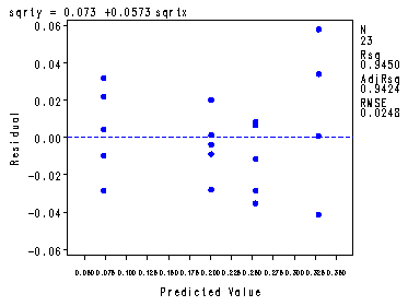
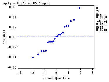
Fig. 3.21, p. 141. Repeating the whole analysis from fig. 3.20 with the transformed response variable.

symbol1 v=dot h=.8 c=blue;
proc reg data =missing;
  model sqrty = x;
  plot r.*p. r.*nqq.;
  output out=temp p=p;
run;
quit;
proc sql;
  create table temp1 as
  select *, (sqrty - mean(sqrty))**2 as sspe1, (mean(sqrty) - p)**2 as sslf1
  from temp
  group by x;
quit;
proc sql;
  create table temp2 as
  select *, sum( sspe1 ) as sspe, sum( sslf1 ) as sslf
  from temp1;
quit;
proc sort data = temp2;
  by sspe sslf;
run; 
data temp3 (keep = sslf sspe mslf mspe f pvalue);
  set temp2;
  by sspe sslf;
  if first.sspe;
  mslf = sslf/2;
  mspe = sspe/19;
  f = (sslf/2) / (sspe/19);
  pvalue = 1 - probf( f, 2, 19);
run;
proc print data = temp3;
 var sslf sspe mslf mspe f pvalue;
run;

The REG Procedure

Model: MODEL1

Dependent Variable: sqrty

                             Analysis of Variance
                                    Sum of           Mean

Source                   DF        Squares         Square    F Value    Pr > F

Model                     1        0.21085        0.21085     188.80    <.0001

Error                    21        0.02345        0.00112

Corrected Total          22        0.23430
Root MSE              0.03342    R-Square     0.8999

Dependent Mean        0.18483    Adj R-Sq     0.8951

Coeff Var            18.08099
                                    Parameter Estimates
                                               Parameter      Standard

Variable    Label                       DF      Estimate         Error   t Value   Pr > |t|

Intercept   Intercept                    1       0.09476       0.00957      9.91     <.0001

x           Plutonium Activity, pCi/g    1       0.01336    0.00097267     13.74     <.0001

Obs      sslf        sspe            mslf          mspe       f           pvalue
 1     0.012106    0.011346    .006053199    .000597174    10.1364    .001009916

Transforming X.

data missing1;
  set missing;
  sqrtx = sqrt(x);
run;

Fig. 3.22a, b and c, p. 142. Repeating the whole analysis from fig. 3.20 with the
transformed response variable and the transformed predictor.

symbol1 v=dot h=.8 c=blue;
proc reg data =missing1;
  model sqrty = sqrtx;
  plot r.*p. r.*nqq.;
  output out=temp p=p;
run;
quit;
proc sql;
  create table temp1 as
  select *, (sqrty - mean(sqrty))**2 as sspe1, (mean(sqrty) - p)**2 as sslf1
  from temp
  group by sqrtx;
quit;
proc sql;
  create table temp2 as
  select *, sum( sspe1 ) as sspe, sum( sslf1 ) as sslf
  from temp1;
quit;
proc sort data = temp2;
  by sspe sslf;
run; 
data temp3 (keep = sslf sspe mslf mspe f pvalue);
  set temp2;
  by sspe sslf;
  if first.sspe;
  mslf = sslf/2;
  mspe = sspe/19;
  f = (sslf/2) / (sspe/19);
  pvalue = 1 - probf( f, 2, 19);
run;
proc print data = temp3;
 var sslf sspe mslf mspe f pvalue;
run;

The REG Procedure

Model: MODEL1

Dependent Variable: sqrty

                             Analysis of Variance
                                    Sum of           Mean

Source                   DF        Squares         Square    F Value    Pr > F

Model                     1        0.22142        0.22142     360.92    <.0001

Error                    21        0.01288     0.00061348

Corrected Total          22        0.23430
Root MSE              0.02477    R-Square     0.9450

Dependent Mean        0.18483    Adj R-Sq     0.9424

Coeff Var            13.40098
                        Parameter Estimates
                     Parameter       Standard

Variable     DF       Estimate          Error    t Value    Pr > |t|

Intercept     1        0.07301        0.00783       9.32      <.0001

sqrtx         1        0.05731        0.00302      19.00      <.0001

Obs          sslf      sspe            mslf          mspe       f        pvalue
 1     .001536829    0.011346    .000768415    .000597174    1.28675    0.29917

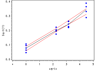
Fig. 3.22d, p. 142.

ods listing close;
proc loess data = missing1;
  model sqrty = sqrtx / degree=2  smooth = .6;
  ods output OutputStatistics=results;
run;
ods listing;
proc sort data = results;
 by sqrtx;
run;
data results1 (rename = ( Depvar=sqrty pred=loess) );
  set results;
run;
proc reg data = results1 noprint;
 model sqrty = sqrtx;
 output out=temp lclm=lower uclm=upper;
run;
quit;
 
symbol1 v=dot i=none c=blue h=.8;
symbol2 v=none i=join c=red line=1;
symbol3 v=none h=.4 i=join c=black line=1;
symbol4 v=none i=join c=red line=1;
axis1 label=(angle=90 'Sqrt(Y)') order=(0 to .4 by .1);
axis2 order=(-1 to 5 by 1);
proc gplot data = temp;
  plot (sqrty lower loess upper)*sqrtx/ overlay vaxis=axis1 haxis=axis2 ;
  format sqrtx 1. sqrty 3.1;
run;
quit;
goptions reset=all;