Applied Linear Statistical Models by Neter, Kutner, et. al. Chapter 6: Multiple Regression I

Inputting the data shown on page 241.

data ch6fig05;
  input x1 x2 y;
  label x1='targtpop'
        x2='dispoinc';
cards;
  68.5  16.7  174.4
  45.2  16.8  164.4
  91.3  18.2  244.2
  47.8  16.3  154.6
  46.9  17.3  181.6
  66.1  18.2  207.5
  49.5  15.9  152.8
  52.0  17.2  163.2
  48.9  16.6  145.4
  38.4  16.0  137.2
  87.9  18.3  241.9
  72.8  17.1  191.1
  88.4  17.4  232.0
  42.9  15.8  145.3
  52.5  17.8  161.1
  85.7  18.4  209.7
  41.3  16.5  146.4
  51.7  16.3  144.0
  89.6  18.1  232.6
  82.7  19.1  224.1
  52.3  16.0  166.5
  ;
run;

Creating the x1x2 variable to be used in Fig. 6.7

data ch6fig05a;
  set ch6fig05;
  x1x2 = x1*x2;
run;

Fig. 6.4a, p. 237.
Scatterplot matrix.
Note: Invoking a macro for the scatter matrix.

%include "c:neter/sas/examples/alsm/scatter.sas";
%scatter(data = ch6fig05a, var = y x1 x2);

Fig. 6.4b, p. 237.
Correlation matrix.

proc corr data = ch6fig05a;
run;

The CORR Procedure

4 Variables: x1 x2 y x1x2

Simple Statistics

Variable N Mean Std Dev Sum Minimum Maximum Label

x1 21 62.01905 18.62033 1302 38.40000 91.30000 targtpop
x2 21 17.14286 0.97035 360.00000 15.80000 19.10000 dispoinc
y 21 181.90476 36.19130 3820 137.20000 244.20000
x1x2 21 1077 373.86333 22609 614.40000 1662

Pearson Correlation Coefficients, N = 21
Prob > |r| under H0: Rho=0

x1 x2 y x1x2

x1 1.00000 0.78130 0.94455 0.99442
targtpop <.0001 <.0001 <.0001

x2 0.78130 1.00000 0.83580 0.83951
dispoinc <.0001 <.0001 <.0001

y 0.94455 0.83580 1.00000 0.95558
<.0001 <.0001 <.0001

x1x2 0.99442 0.83951 0.95558 1.00000
<.0001 <.0001 <.0001

Fig. 6.5a and b, p. 241.
Note that output statement is used to create outfig05 with fitted and residual values.

proc reg data = ch6fig05a;
  var x1x2;
  model y = x1 x2/ i;
  output out=outfig05 p = fitted r = residual;
run;
quit;

The REG Procedure
Model: MODEL1
Dependent Variable: y

X’X Inverse, Parameter Estimates, and SSE

Variable Label Intercept x1 x2 y

Intercept Intercept 29.728923483 0.0721834719 -1.992553186 -68.85707315
x1 targtpop 0.0721834719 0.0003701761 -0.005549917 1.4545595828
x2 dispoinc -1.992553186 -0.005549917 0.1363106368 9.3655003765
y -68.85707315 1.4545595828 9.3655003765 2180.9274114

Analysis of Variance

Sum of Mean
Source DF Squares Square F Value Pr > F

Model 2 24015 12008 99.10 <.0001
Error 18 2180.92741 121.16263
Corrected Total 20 26196

Root MSE 11.00739 R-Square 0.9167
Dependent Mean 181.90476 Adj R-Sq 0.9075
Coeff Var 6.05118

Parameter Estimates

Parameter Standard
Variable Label DF Estimate Error t Value Pr > |t|

Intercept Intercept 1 -68.85707 60.01695 -1.15 0.2663
x1 targtpop 1 1.45456 0.21178 6.87 <.0001
x2 dispoinc 1 9.36550 4.06396 2.30 0.0333

Show all variables, including fitted and residual as shown in Fig. 6.5b, p. 24

proc print data = outfig05;
  var y x1 x2 fitted residual;
run;

Obs y x1 x2 fitted residual

1 174.4 68.5 16.7 187.184 -12.7841
2 164.4 45.2 16.8 154.229 10.1706
3 244.2 91.3 18.2 234.396 9.8037
4 154.6 47.8 16.3 153.329 1.2715
5 181.6 46.9 17.3 161.385 20.2151
6 207.5 66.1 18.2 197.741 9.7586
7 152.8 49.5 15.9 152.055 0.7449
8 163.2 52.0 17.2 167.867 -4.6666
9 145.4 48.9 16.6 157.738 -12.3382
10 137.2 38.4 16.0 136.846 0.3540
11 241.9 87.9 18.3 230.387 11.5126
12 191.1 72.8 17.1 197.185 -6.0849
13 232.0 88.4 17.4 222.686 9.3143
14 145.3 42.9 15.8 141.518 3.7816
15 161.1 52.5 17.8 174.213 -13.1132
16 209.7 85.7 18.4 228.124 -18.4239
17 146.4 41.3 16.5 145.747 0.6530
18 144.0 51.7 16.3 159.001 -15.0013
19 232.6 89.6 18.1 230.987 1.6130
20 224.1 82.7 19.1 230.316 -6.2161
21 166.5 52.3 16.0 157.064 9.4356

Note: To recreate the 3-D plots in Fig. 6.6 use interactive data analysis in SAS,

visit our web page https://stats.idre.ucla.edu/stat/sas/teach/reg_int/reg_int_cont.htm
.

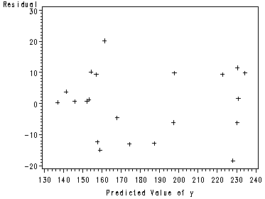
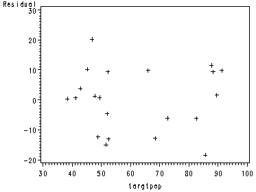
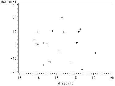
Fig. 6.7, p. 246, showing 4 different diagnostic plots.

proc gplot data = outfig05;
  plot residual*fitted;
run;

proc gplot data = outfig05;
  plot residual*x1;
run;

proc gplot data = outfig05;
  plot residual*x2;
run;

proc gplot data = outfig05;
  plot residual*x1x2;
run;

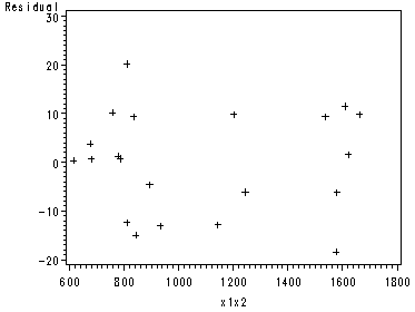
Fig 6.8a-Fig 6.8d, page 247 could have been obtained all
in one proc gplot command as shown below.

proc gplot data = outfig05;
  plot residual*fitted;
  plot residual*x1;
  plot residual*x2;
  plot residual*x1x2;
run;

Fig 6.8a, page 247.

data outfig08;
  set outfig05;
  absresid = abs(residual);
run;
 
proc gplot data=outfig08;
  plot absresid*fitted;
run;

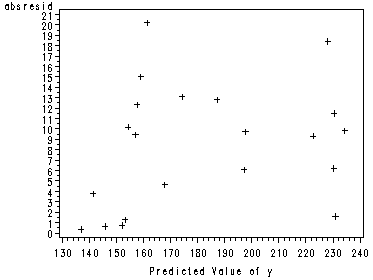
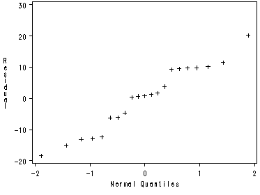
Fig. 6.8b, p. 247, normal probability plot.
Note: The labels on the X-axis differs from the book.

proc univariate data = outfig05 noprint ;
  qqplot residual / normal;
run;

Estimation of Mean Response and Prediction Limits for New Observations, p. 249-251.
Adding an extra line of data in order to predict.

data ch6fig05h;
  input x1 x2 y;
cards;
  68.5  16.7  174.4
  45.2  16.8  164.4
  91.3  18.2  244.2
  47.8  16.3  154.6
  46.9  17.3  181.6
  66.1  18.2  207.5
  49.5  15.9  152.8
  52.0  17.2  163.2
  48.9  16.6  145.4
  38.4  16.0  137.2
  87.9  18.3  241.9
  72.8  17.1  191.1
  88.4  17.4  232.0
  42.9  15.8  145.3
  52.5  17.8  161.1
  85.7  18.4  209.7
  41.3  16.5  146.4
  51.7  16.3  144.0
  89.6  18.1  232.6
  82.7  19.1  224.1
  52.3  16.0  166.5
  65.4  17.6    .  
  53.1  17.7    .  
  ;
run;

Getting the predicted value and the CI’s for E[Yh] and Yh(new), p. 249-251.
Upper and Lower CLMean is for E[Yh] and Upper and Lower CL is for Yh(new).

proc reg data = ch6fig05h  ;
  model y = x1 x2 / r cli clm;
  ods output OutputStatistics=temp;
run;
quit;

The REG Procedure
Model: MODEL1
Dependent Variable: y

Analysis of Variance

Sum of Mean
Source DF Squares Square F Value Pr > F

Model 2 24015 12008 99.10 <.0001
Error 18 2180.92741 121.16263
Corrected Total 20 26196

Root MSE 11.00739 R-Square 0.9167
Dependent Mean 181.90476 Adj R-Sq 0.9075
Coeff Var 6.05118

Parameter Estimates

Parameter Standard
Variable DF Estimate Error t Value Pr > |t|

Intercept 1 -68.85707 60.01695 -1.15 0.2663
x1 1 1.45456 0.21178 6.87 <.0001
x2 1 9.36550 4.06396 2.30 0.0333

The REG Procedure
Model: MODEL1
Dependent Variable: y

Output Statistics

Dep Var Predicted Std Error
Obs y Value Mean Predict 95% CL Mean 95% CL Predict Residual

1 174.4000 187.1841 2 164.4000 154.2294 3 244.2000 234.3963 4 154.6000 153.3285 5 181.6000 161.3849 6 207.5000 197.7414 7 152.8000 152.0551 8 163.2000 167.8666 9 145.4000 157.7382 10 137.2000 136.8460 11 241.9000 230.3874 12 191.1000 197.1849 13 232.0000 222.6857 14 145.3000 141.5184 15 161.1000 174.2132 16 209.7000 228.1239 17 146.4000 145.7470 18 144.0000 159.0013 19 232.6000 230.9870 20 224.1000 230.3161 21 166.5000 157.0644 22 . 191.1039 23 . 174.1494 3.8409 179.1146 195.2536 162.6910 211.6772 -12.7841
3.5558 146.7591 161.6998 129.9271 178.5317 10.1706
4.5882 224.7569 244.0358 209.3421 259.4506 9.8037
3.2331 146.5361 160.1210 129.2260 177.4311 1.2715
4.4300 152.0778 170.6921 136.4566 186.3132 20.2151
4.3786 188.5424 206.9404 172.8533 222.6295 9.7586
4.1696 143.2952 160.8150 127.3259 176.7843 0.7449
3.3310 160.8684 174.8649 143.7053 192.0280 -4.6666
2.9628 151.5136 163.9628 133.7895 181.6869 -12.3382
4.0074 128.4268 145.2653 112.2354 161.4566 0.3540
4.2012 221.5610 239.2137 205.6346 255.1402 11.5126
3.4109 190.0188 204.3510 172.9744 221.3954 -6.0849
5.3808 211.3810 233.9904 196.9448 248.4266 9.3143
4.1735 132.7502 150.2866 116.7863 166.2506 3.7816
5.0377 163.6294 184.7971 148.7807 199.6458 -13.1132
4.1214 219.4652 236.7826 203.4304 252.8174 -18.4239
3.7331 137.9041 153.5899 121.3276 170.1664 0.6530
3.2529 152.1672 165.8354 134.8870 183.1157 -15.0013
4.4176 221.7059 240.2681 206.0684 255.9056 1.6130
5.8120 218.1054 242.5267 204.1647 256.4675 -6.2161
4.0792 148.4944 165.6344 132.4018 181.7270 9.4356
2.7668 185.2911 196.9168 167.2589 214.9490 .
4.5986 164.4881 183.8107 149.0867 199.2121 .

Output Statistics

Std Error Student Cook’s
Obs Residual Residual -2-1 0 1 2 D

1 10.316 -1.239 | **| | 0.071
2 10.417 0.976 | |* | 0.037
3 10.006 0.980 | |* | 0.067
4 10.522 0.121 | | | 0.000
5 10.077 2.006 | |**** | 0.259
6 10.099 0.966 | |* | 0.059
7 10.187 0.0731 | | | 0.000
8 10.491 -0.445 | | | 0.007
9 10.601 -1.164 | **| | 0.035
10 10.252 0.0345 | | | 0.000
11 10.174 1.132 | |** | 0.073
12 10.466 -0.581 | *| | 0.012
13 9.603 0.970 | |* | 0.098
14 10.186 0.371 | | | 0.008
15 9.787 -1.340 | **| | 0.159
16 10.207 -1.805 | ***| | 0.177

The REG Procedure
Model: MODEL1
Dependent Variable: y

Output Statistics

Std Error Student Cook’s
Obs Residual Residual -2-1 0 1 2 D

17 10.355 0.0631 | | | 0.000
18 10.516 -1.427 | **| | 0.065
19 10.082 0.160 | | | 0.002
20 9.348 -0.665 | *| | 0.057
21 10.224 0.923 | |* | 0.045
22 . . .
23 . . .

Sum of Residuals 0
Sum of Squared Residuals 2180.92741
Predicted Residual SS (PRESS) 3002.92331

We use Where Observation >= 22 to show just the last two observation

proc print data = temp;
  where Observation >= 22;
run;

StdErr
Predicted Mean Lower Upper
Obs Model Dependent Observation DepVar Value Predict CLMean CLMean

22 MODEL1 y 22 . 191.1039 2.7668 185.2911 196.9168
23 MODEL1 y 23 . 174.1494 4.5986 164.4881 183.8107

StdErr Student
Obs LowerCL UpperCL Residual Residual Residual Picture CooksD

22 167.2589 214.9490 . . . .
23 149.0867 199.2121 . . . .