Applied Regression Analysis by John Fox Chapter 14: Extending Linear Least Squares…

Section 14.1 Time Series Regression and Generalized Least Squares

Figure 14. 3. on page 380 using data file
hartnagl.

proc sort data = hartnagl;
  by year;
run;
symbol1 c=black v=star i = join h=0.5;
title 'Figure 14.3.';
filename outfiles 'https://stats.idre.ucla.edu/wp-content/uploads/2016/02/chp14Fig3.gif';
axis1 order = (1935 to 1970 by 5);
axis2 order = (0 to 75 by 25) label = (r = 0 a =90);
proc gplot data = hartnagl;
  plot ftheft*year /haxis=axis1 vaxis=axis2 vminor= 0 hminor =0;
  label year='Year';
  label ftheft ='Theft Convictions per 100,000';
run;
quit;

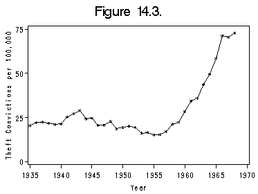
Table 14.1. The OLS column using proc reg. We use the
option dw to get the first order autocorrelation which will be
used later in this section.

proc reg data=hartnagl;  /*This is the first column of Table 14.1*/
  model ftheft = fertil labor postsec mtheft/dw;
  output out=hartreg p=p r=r;
  run;
quit;

The REG Procedure
Model: MODEL1
Dependent Variable: ftheft

                        Analysis of Variance
                        
		        (Output omitted here.)
                        Parameter Estimates

                     Parameter       Standard
Variable     DF       Estimate          Error    t Value    Pr > |t|
Intercept     1       -7.33414        9.43792      -0.78      0.4434
fertil        1       -0.00609        0.00145      -4.20      0.0002
labor         1        0.11994        0.02341       5.12      <.0001
postsec       1        0.55156        0.04325      12.75      <.0001
mtheft        1        0.03932        0.01856       2.12      0.0428
Durbin-Watson D                1.424
Number of Observations            34
1st Order Autocorrelation      0.244

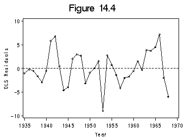
Figure 14.4 on page 381 on residuals from the above OLS
regression.

title 'Figure 14.4';
symbol color=black i=join  v=star h=0.5; 
axis1 order = (1935 to 1970 by 5);
axis2 order =(-10 to 10 by 5) label =(r=0 a=90);

proc gplot data=hartreg;
  plot r*year =1 /haxis=axis1 vaxis=axis2 vminor=0 hminor=0 vref=0 lvref=2;
  label r='OLS Residuals';
  label year ='Year';
run;
quit;

Second column of Table 14.1: EGLS(1).

data hartnew; /*transform data based on [14.7];*/
  set hartnagl (firstobs=5); /*omit missing data*/
  ftheft1= ftheft-0.244*lag(ftheft);
  fertil1 = fertil-0.244*lag(fertil);
  labor1 = labor-0.244*lag(labor);
  postsec1 = postsec -0.244*lag(postsec);
  mtheft1 = mtheft - 0.244*lag(mtheft);
  const=.756;
  if _n_ eq 1 then do;
    ftheft1 = sqrt(1-.244*.244)*ftheft;
    fertil1 = sqrt(1-.244*.244)*fertil;
    labor1 = sqrt(1-.244*.244)*labor;
    postsec1 = sqrt(1-.244*.244)*postsec;
    mtheft1 = sqrt(1-.244*.244)*mtheft;
    const = sqrt(1-.244*.244);
  end;
run;
proc reg data=hartnew ;    /*second column of Table 14.1*/
  model ftheft1 =const fertil1 labor1 postsec1 mtheft1/ noint dw;
  output out=hartreg p=p r=r;
  run;
quit;


The REG Procedure
Model: MODEL1
Dependent Variable: ftheft1

NOTE: No intercept in model. R-Square is redefined.

                        Analysis of Variance
                        (Output omtted here.)
                        Parameter Estimates

                     Parameter       Standard
Variable     DF       Estimate          Error    t Value    Pr > |t|

const         1       -6.64294       11.12007      -0.60      0.5549
fertil1       1       -0.00588        0.00178      -3.30      0.0025
labor1        1        0.11563        0.02709       4.27      0.0002
postsec1      1        0.53588        0.05005      10.71      <.0001
mtheft1       1        0.03993        0.02198       1.82      0.0796

Column EGLS(2) of Table 14.1.

proc reg data=hartnew (firstobs=2); /*third column of Table 14.1*/
  model ftheft1 = const fertil1 labor1 postsec1 mtheft1/ noint dw;
  run;
quit;


The REG Procedure
Model: MODEL1
Dependent Variable: ftheft1

NOTE: No intercept in model. R-Square is redefined.

                        Analysis of Variance
                        (Output omitted.)  
                        
                        Parameter Estimates

                     Parameter       Standard
Variable     DF       Estimate          Error    t Value    Pr > |t|
const         1       -5.51854       11.73656      -0.47      0.6419
fertil1       1       -0.00608        0.00189      -3.21      0.0033
labor1        1        0.11365        0.02808       4.05      0.0004
postsec1      1        0.53421        0.05104      10.47      <.0001
mtheft1       1        0.04071        0.02242       1.82      0.0802

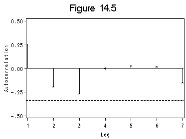
Figure 14.5 on residual autocorrelations from the OLS regression. The output from proc autoreg is omitted here.

proc autoreg data=hartnagl(firstobs=5); 
  model ftheft = fertil labor postsec mtheft/ nlag = 7 dw=7;
  ods  output CorrGraph=hartautoreg;
  run;
quit;

proc univariate data=hartautoreg (firstobs=2); /*for standard error of Autocorr;*/
  var Autocorr;
run;

axis1 order =(1 to 7 by 1);
axis2 order =(-0.5 to 0.5 by 0.25) label=(r=0 a=90);
symbol1 color=black i=needle v=star height=0.5;
title 'Figure 14.5';
proc gplot data=hartautoreg(firstobs=2);
  format Autocorr 4.2;
  plot Autocorr*Lag=1/ haxis=axis1 vaxis=axis2 
  hminor=0 vminor=0 vref=(-0.342 0 0.342) lvref=2;/*standard error obtained from */ 
  /*proc univariate before*/
  label Autocorr='Autocorrelation';     
run;
quit;

Section 14.2 Nonlinear Regression

Figure 14.9 on page 400 using data file uspop.
We use proc nlin to build the logistic model. See the output of proc nlin below.

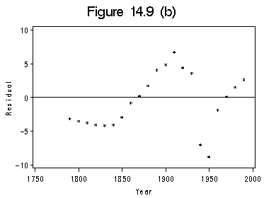
proc nlin data=uspop;
  parms b1=350 b2=4.5  b3=-0.3;
  model pop = b1/(1+exp(b2+b3*(year-1790)));
  output out=mypred p=pred r=res;
  run;
quit;

title 'Figure 14.9 (a)';
axis1 order=(1750 to 2000 by 50);
axis2 order=(0 to 300 by 100) label=(r=0 a=90);
symbol1 c=black i=none v=star h=0.5;
symbol2 c=blue i=spline v=none h=0.8;
proc gplot data=mypred;
  plot pop*year=1 pred*year=2/overlay haxis=axis1 vaxis=axis2 hminor=0 vminor=0;
  label year='Year';
  label pop='Population in Million';
run;
quit;

title 'Figure 14.9 (b)';
axis1 order=(1750 to 2000 by 50);
axis2 order=(-10 to 10 by 5) label=(r=0 a=90);
symbol1 c=black i=none v=star h=0.5;
proc gplot data=mypred;
  plot res*year=1 /haxis=axis1 vaxis=axis2 hminor=0 vminor=0 vref=0;
  label year='Year';
  label res='Residual';
run;
quit;

The NLIN Procedure
Iterative Phase
Dependent Variable pop
Method: Gauss-Newton

Sum of
Iter b1 b2 b3 Squares
0 350.0 4.5000 -0.3000 1312135
1 100.4 3.1027 -0.1468 97469.7
...more iterations...
11 389.2 3.9903 -0.0227 356.4
12 389.2 3.9903 -0.0227 356.4

NOTE: Convergence criterion met.
Estimation Summary
Method Gauss-Newton
Iterations 12
Subiterations 8
Average Subiterations 0.666667
R 2.52E-6
PPC(b3) 2.873E-7
RPC(b1) 0.000011
Object 1.123E-9
Objective 356.4001
Observations Read 21
Observations Used 21
Observations Missing 0

NOTE: An intercept was not specified for this model.
Sum of Mean Approx
Source DF Squares Square F Value Pr > F
Regression 3 277075 92358.3 4664.56 <.0001
Residual 18 356.4 19.8000
Uncorrected Total 21 277431

Corrected Total 20 123094
The NLIN Procedure

Approx
Parameter Estimate Std Error Approximate 95% Confidence Limits
b1 389.2 30.8120 324.4 453.9
b2 3.9903 0.0703 3.8426 4.1381
b3 -0.0227 0.00109 -0.0249 -0.0204
Approximate Correlation Matrix
b1 b2 b3
b1 1.0000000 -0.1662420 0.9145422
b2 -0.1662420 1.0000000 -0.5406525
b3 0.9145422 -0.5406525 1.0000000

Section 14.3 Robust Regression

Table 14.8 on different M-estimates using data file
duncan.
SAS is not very strong at iterated reweighted least squares (IRLS). The way
SAS does it is to use proc nlin. On the other hand Stata has procedures
such as rreg (robust regression) that do IRLS nicely. Please refer to our
corresponding Stata page of this section for more details.

proc reg data=duncan;  /*Least squares*/
  model prestige=income educ;
run;
quit;
proc reg data=duncan; /*Least sqaures with two extreme obs omitted*/
  model prestige = income educ;
  where (occtitle ne 'minister' and occtitle ne 'railroad_conductor');
run;
quit;
data duncan1;
  set duncan;
  cons = 1;
run;

proc iml; /*Least absolute values*/
  use duncan1;
  read all;
 
  a = cons || income || educ;
  b=prestige;
  call lav(rc,xr,a,b,);
  print xr;  /*This gives the regression coefficient.*/
run;
quit;

The REG Procedure: Least Squares
Model: MODEL1
Dependent Variable: prestige

                        Analysis of Variance
                         (Output omitted.)
                        Parameter Estimates

                     Parameter       Standard
Variable     DF       Estimate          Error    t Value    Pr > |t|
Intercept     1       -6.06466        4.27194      -1.42      0.1631
income        1        0.59873        0.11967       5.00      <.0001
educ          1        0.54583        0.09825       5.56      <.0001

The REG Procedure: Least Squares*
Model: MODEL1
Dependent Variable: prestige

                        Analysis of Variance
                         (Output omitted.)
                        Parameter Estimates

                     Parameter       Standard
Variable     DF       Estimate          Error    t Value    Pr > |t|
Intercept     1       -6.40899        3.65263      -1.75      0.0870
income        1        0.86740        0.12198       7.11      <.0001
educ          1        0.33224        0.09875       3.36      0.0017

Least Absolute Values
                               
                             LAV (L1) Estimation
                             Start with LS Solution
                       Start Iter: gamma=34.64122528 ActEqn=45
    Iter     N Huber     Act Eqn        Rank       Gamma         L1(x)      F(Gamma)
       1           1           7           3      1.6741    435.454385    399.879402
                ...more iterations...
       6           8           3           3      0.0000    415.977064    412.655271

Algorithm converged
Objective Function L1(x)= 415.97706422
Number Search Directions=       15
Number Refactorizations =        4
Total Execution Time=       0.0000

XR
-6.408257 0.7477064 0.4587156

Section 14.4 Nonparametric Regression

Figure 14.15 on page 418 using data file prestige.

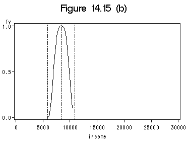
proc sort data=prestige;
  by income;
run;

proc print data=prestige (firstobs=80 obs=80); /*to get income[80]*/
  var income;
run;

data pre1; /*start to create the neighborhood around income[80]*/
  set prestige;
  neb = abs(income-8403);
run;

proc sort data=pre1;
  by neb;
run;

data preseg;
  set pre1;
  if _n_ le 40;
  output;
run; /*done creating the neighborhood*/
proc sort data=preseg;
  by income;
run;

proc print data=preseg (firstobs=1 obs=1);/*this gives the lower reference line*/
  var income;
run;

proc print data =preseg (firstobs=40 obs=40);/*this gives the upper reference line*/
  var income;
run;

title 'Figure 14.15 (a)';
axis1 order =(0 to 30000 by 5000);
axis2 order=(0 to 1 by 0.5) label =(r=0 a=90);
symbol1 c = black i=none v=star h=0.8;
proc gplot data=prestige;
  plot prestige*income=1 /hminor=0 vminor=0 href=(5902 8403 10904) lhref=2;
  label income='Average Income, Dollars';
  label prestige='Prestige';
run;
quit;

data preseg1;
  set preseg;
  stinc=abs(income-8403)/2501;
  fv=(1-abs(stinc)**3)**3;
  if fv < 0 then  fv=0;
run;

proc sort data=preseg1;
  by income;
run;

title 'Figure 14.15 (b)';
filename outfiles 'https://stats.idre.ucla.edu/wp-content/uploads/2016/02/chp14Fig15b.gif';
axis1 order =(0 to 30000 by 5000);
axis2 order=(0 to 1 by 0.5);
symbol1 c = black i=join v=none h=0.8;
proc gplot data=preseg1;
  plot fv*income=1 / haxis=axis1 vaxis=axis2 hminor=0 vminor=0 
  href=(5902 8403 10904)  lhref=2;
run;
quit;

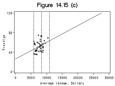
title 'Figure 14.15 (c)';
filename outfiles 'https://stats.idre.ucla.edu/wp-content/uploads/2016/02/chp14Fig15c.gif';
axis1 order =(0 to 30000 by 5000);
axis2 order=(0 to 120 by 40) label=(r=0 a=90);
symbol1 c = black i=rls v=star h=0.8; /*using the option i=rls to get regression line*/
proc gplot data=preseg;
  plot prestige*income=1 /haxis=axis1 vaxis=axis2 hminor=0 vminor=0 
  href=(5902 8403 10904) lhref=2;
  label income='Average Income, Dollars';
  label prestige='Prestige';
run;
quit;

proc loess data=prestige;
  model prestige=income /smooth=0.4;
  ods output OutputStatistics=myout;
  run;
quit;
proc sort data=myout;
  by income;
run;
title 'Figure 14.15 (d)';
filename outfiles 'https://stats.idre.ucla.edu/wp-content/uploads/2016/02/chp14Fig15d.gif';
axis1 order =(0 to 30000 by 5000);
axis2 order=(0 to 120 by 40) label=(r=0 a=90);
symbol1 c = black i=none v=star h=0.8;
symbol2 c=blue i=join v=none h=0.8;
proc gplot data=myout;
  format DepVar f4.0 income f8.0;
  plot DepVar*income=1 Pred*income=2 /overlay haxis=axis1 vaxis=axis2 hminor=0 vminor=0;
  label income='Average Income, Dollars';
  label DepVar='Prestige';
run;
quit;

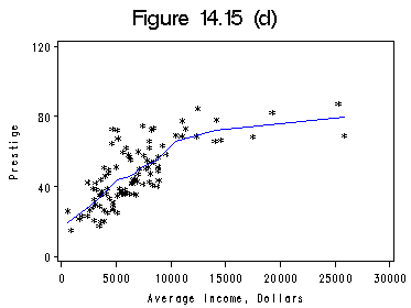
Figure 14.16 on page 421 showing lowess regression and
its residuals.

proc loess data=prestige;
  model prestige=income /smooth=0.5 all; /*This actually is the default. */
  ods output OutputStatistics=myout1;
  run;
quit;

proc sort data=myout1;
  by income;
run;

title 'Figure 14.16 (a)';
filename outfiles 'https://stats.idre.ucla.edu/wp-content/uploads/2016/02/chp14Fig16a.gif';
axis1 order =(0 to 30000 by 5000);
axis2 order=(0 to 120 by 40) label=(r=0 a=90);
symbol1 c = black i=none v=star h=0.8;
symbol2 c=blue i=join v=none h=0.8;
proc gplot data=myout1;
  format DepVar f4.0 income f8.0;
  plot DepVar*income=1 Pred*income=2 /overlay haxis=axis1 vaxis=axis2 hminor=0 vminor=0;
  label income='Average Income, Dollars';
  label DepVar='Prestige';
run;
quit;

proc loess data=myout1;
  model Residual=income /smooth=0.5;
  ods output OutputStatistics=resout;
  run;
quit;

proc sort data=resout;
  by income;
run;

title 'Figure 14.16 (b)';
filename outfiles 'https://stats.idre.ucla.edu/wp-content/uploads/2016/02/chp14Fig16b.gif';
axis1 order =(0 to 30000 by 5000);
axis2 order=(-25 to 50 by 25) label=(r=0 a=90);
symbol1 c = black i=none v=star h=0.8;
symbol2 c=blue i=join v=none h=0.8;
proc gplot data=resout;
  format DepVar f4.0 income f8.0;
  plot DepVar*income=1 Pred*income=2 /overlay haxis=axis1 
  vaxis=axis2 hminor=0 vminor=0 vref=0 lvref=2;
  label income='Average Income, Dollars';
  label DepVar='Lowess Residual';
run;
quit;

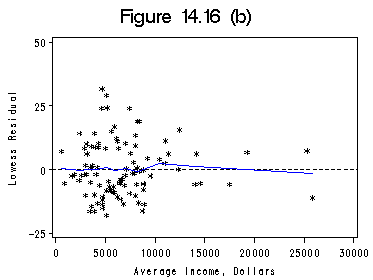
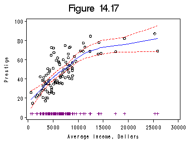
Figure 14.17 on lowess regression with 95% confidence
envelope for the lowess smooth. Figure 14.18 can be done in exactly the same
way. proc loess does lowess smoothing with option all
giving the 95% confidence envelope.

proc loess data=prestige;
  ods output OutputStatistics = pres
  FitSummary=Summary; 
  model prestige = income /  direct smooth = 0.6667 all;
run;
quit
;
proc sort data=pres;
  by income;
run;

data pres1; /*to create a variable for one-way plot*/
  set pres;
  oneway=4;
run;

title 'Figure 14.17';
filename outfiles 'https://stats.idre.ucla.edu/wp-content/uploads/2016/02/chp14Fig17.gif';
axis1 order=(0 to 30000 by 5000);
axis2 order =(0 to 100 by 20) label=(r=0 a=90);
symbol1 c=black i=none v=circle h=0.8;
symbol2 c=blue i=join v=none h=0.8;
symbol3 c=red i=join v= none line=2 h=0.8;
symbol4 c=purple i=none v='|' h=1;
proc gplot data=pres1;
  format DepVar f4.0 income f6.0;
  plot DepVar*income=1 Pred*income=2 (LowerCL UpperCL)*income=3 oneway*income=4 
  /overlay haxis=axis1 vaxis=axis2 hminor=0 vminor=0;
  label income='Average Income, Dollars';
  label DepVar='Prestige';
run;
quit;