Section 15.1 Models for Dichotomous Data
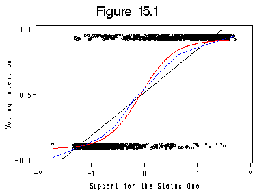
Figure 15.1. using data file chile.
data chilenew; /*jittered dataset*/
  set chile;
  if (intvote = 2) then voting = 0;
  else voting = 1;
  vjitter = voting  + 0.05*ranuni(0);
  if(intvote <3); /*1 for and 2 against*/
  output;
  run;
proc logistsic data=chilenew descending noprint; /*descending option is needed*/
  model voting=statquo;
  output out=chile1 predicted=lpred; /*output data file for further analysis*/
  run;
proc loess data=chile1;
  model voting=statquo;
  ods output PredAtVertices=chile2;
  run;
proc sort data=chile2;
  by statquo;
proc sort data=chile1;
  by statquo;
run;
data chile3;
  merge chile1 chile2;
  by statquo;
  run;

goptions gsfname=outfiles dev=gif373;
symbol1 c=black i=rls v=circle h=0.5;
symbol2 c=red i=join v=none;
symbol3 c=blue i=join v=none h=0.5 line=2;
title 'Figure 15.1';
filename outfiles 'https://stats.idre.ucla.edu/wp-content/uploads/2016/02/chp15Fig1.gif';
axis1 order = (-2 to 2 by 1);
axis2 order = (-0.1 to 1.1 by 0.6) label=(r=0 a=90);;
proc gplot data=chile3;
  format statquo f2.0;
  plot vjitter*statquo=1 lpred*statquo=2 Pred*statquo=3 / haxis=axis1
       vaxis=axis2 overlay vminor=0 hminor=0;
  label statquo='Support for the Status Quo';
  label vjitter='Voting Intention';
  run;
quit;
Table 15.1 and Table 15.2 on page 452 using data file womenlf. In order to use proc logistic correctly, dummy variables are created to present the status of working, the presence of children and the region. The deviance in the table is -2*Log L which is presented in the output. The (G0)2 in Table 15.2 is the difference of -2*Log L between the two models being compared. The p-value is then obtained using chi-square distribution with the corresponding degree of freedom. On the other hand, proc logistic uses Wald-test (shown below) instead of (G0)2.
data wcoded;
  set womenlf;
  if (work='not_work') then wstatus=0;
  else wstatus =1;
  if (child ='present') then kid = 1;
  else kid =0;
  if (region ='Ontario') then re1= 1;
  else re1 =0;
  if (region ='Prairie') then re2=1;
  else re2=0;
  if (region ='Atlantic') then re3=1;
  else re3=0;
  if (region = 'Quebec') then re4=1;
  else re4=0;
  ik=husbinc*kid;
  run;
proc logistic data=wcoded;/*model 1*/
  model wstatus = husbinc kid re1-re4 ik;
  test2: test ik;/* model contrast:2-1*/
  test5: test re1, re2, re3, re4;/*model contrast : 3-1*/
  run;
proc logistic data=wcoded; /*model 2*/
  model wstatus = husbinc kid re1-re4;
  test3: test husbinc;/*model contrast: 5-2*/
  test4: test kid; /*model contrast: 4-2 */
  run;
proc logistic data=wcoded; /*model 3*/
  model wstatus = husbinc kid ik;
  run;
proc logistic data=wcoded; /*model 4*/
  model wstatus = husbinc  re1-re4;
  run;
proc logistic data=wcoded;/*model 5*/
  model wstatus = kid re1-re4;
  run;
The LOGISTIC Procedure ---Model 1---

    (Output omitted here.)

             Model Fit Statistics For Model 1

                              Intercept
               Intercept         and
Criterion        Only        Covariates
AIC              358.151        332.542
SC               361.723        361.119
-2 Log L         356.151        316.542

              Testing Global Null Hypothesis: BETA=0

     Test                 Chi-Square       DF     Pr > ChiSq

    Likelihood Ratio        39.6094        7         <.0001
    Score                   38.6566        7         <.0001
    Wald                    33.8338        7         <.0001

        Linear Hypotheses Testing Results

                Wald
 Label    Chi-Square      DF    Pr > ChiSq
 TEST2        0.7547       1        0.3850 --comparing model 2 with model 1
 TEST5        2.5477       4        0.6361 --comparing model 3 with model 1

    The LOGISTIC Procedure ---Model 2---

    (Output omitted here.)

               Model Fit Statistics For Model 2

                              Intercept
               Intercept         and
Criterion        Only        Covariates
AIC              358.151        331.301
SC               361.723        356.306
-2 Log L         356.151        317.301

        Linear Hypotheses Testing Results

                Wald
 Label    Chi-Square      DF    Pr > ChiSq
 TEST3        4.8567       1        0.0275 --comparing model 5 and model 2
 TEST4       28.2452       1        <.0001 --comparing model 4 and model 2

    The LOGISTIC Procedure ---Model 3---

    (Output omitted here.)

         Model Fit Statistics

                              Intercept
               Intercept         and
Criterion        Only        Covariates
AIC              358.151        327.124
SC               361.723        341.413
-2 Log L         356.151        319.124

    The LOGISTIC Procedure ---Model 4---

(Output omitted here.)

         Model Fit Statistics

                              Intercept
               Intercept         and
Criterion        Only        Covariates
AIC              358.151        359.849
SC               361.723        381.282
-2 Log L         356.151        347.849

The LOGISTIC Procedure ---Model 5---

(Output omitted here.)

         Model Fit Statistics

                              Intercept
               Intercept         and
Criterion        Only        Covariates
AIC              358.151        334.427
SC               361.723        355.860
-2 Log L         356.151        322.427
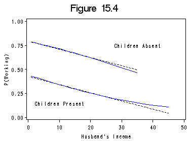
Figure 15.4 on page 453.
proc logistic data= wcoded  descending noprint;
  model wstatus = kid husbinc /rsquare;
  output out=women predicted=pred;
run;

proc reg data=women noprint;
  model wstatus = husbinc kid;
  output out = women1 predicted=lpr;
run;

data women2; /*to create a dataset for gplot */
  set women1;
  if (kid=1) then do l1=lpr; p1=pred; end;
  else do l2=lpr; p2=pred; end;
  output;
run;

proc sort data=women2;
  by husbinc;
run;

data labels; /*for the text in the graph*/
  length function style $ 8 text $17;
  retain function 'label' xsys  ysys '2' when 'a' color 'black';
  function='label'; x=10; y=0.15; size=1; color='black'; text='Children Present'; output;
  function='label'; x=35; y=0.75; size=1; color='black'; text='Children Absent'; output;
run;

title 'Figure 15.4';
symbol1 c=black i=join v=none h=1 line=2;
symbol2 c=blue i=join v=none h=1 line=1;
axis1 order =(0 to 50 by 10);
axis2 order=(0 to 1 by .25) label=(r=0 a=90);
proc gplot data=women2;
  plot l1*husbinc=1 l2*husbinc=1 p1*husbinc=2 p2*husbinc=2
        / annotate=labels haxis=axis1 vaxis=axis2 hminor=0 vminor=0 overlay;
  label husbinc='Husband''s Income';
  label l1='P(Working)';
run;
quit;
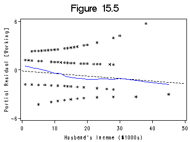
Figure 15.5 on page 459 using the same data file womenlf as above.
data wcoded1;
  set womenlf;
  if (work='not_work') then do w=2; wstatus=1; end;
  else if (work='fulltime') then do w=0; wstatus=0; end;
  else do w=1; wstatus =0; end;
  if (child ='present') then kid = 1;
  else kid =0;
  if (region ='Ontario') then re1= 1;
  else re1 =0;
  if (region ='Prairie') then re2=1;
  else re2=0;
  if (region ='Atlantic') then re3=1;
  else re3=0;
  if (region = 'Quebec') then re4=1;
  else re4=0;
  ik=husbinc*kid;
  run;

proc logistic data=wcoded1 descending noprint;
  model wstatus =husbinc kid ;
  output out=women predicted=pr;
run;

data women1; /*to create partial residuals*/
  set women;
  rh = (pr-wstatus)/(pr*(1-pr)) -0.0423*husbinc;
run;

proc loess data=women1;/*to create data for lowess smooth of the plot*/
  model rh=husbinc /iterations=2 direct smooth=0.5; /*set iterations to be 2 for outliers*/
  ods output OutputStatistics=women2;
run;

proc sort data=women1;
  by husbinc;
run;

proc sort data=women2;
  by husbinc;
run;

data women3;
  merge women1 women2;
  by husbinc;
run;

title 'Figure 15.5';
symbol1 color=black i=rls v=star h=0.8 line=2;
symbol2 color=blue i=jone v=none h=1 line =1;
axis1 order=(0 to 50 by 10);
axis2 order=(-6 to 6 by 6) label=(r=0 a=90);
proc gplot data=women3;
  format husbinc f4.0;
  plot rh*husbinc=1 Pred*husbinc=2/ overlay haxis=axis1 vaxis=axis2 vminor=0 hminor=0;
  label husbinc='Husband''s Income ($1000s)';
  label rh='Partial Residual [Working]';
run;
quit;
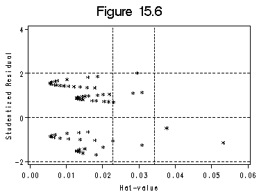
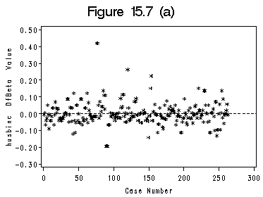
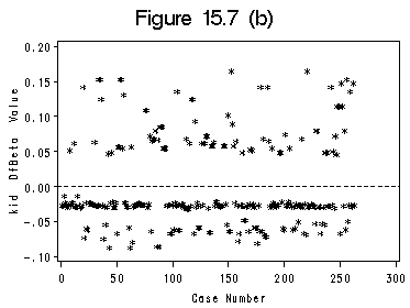
Figure 15.6 and Figure 15.7 (a) and (b). We use SAS ODS to output the influence statistics to a data file. Index plots of Dfbeta are basically the plots presented in Figure (a) and (b).
proc logistic data=wcoded;
  model wstatus=husbinc kid/influence ;
  ods output Influence=winf;
run;

data winf1;
  set winf;
  g=ResDev/sqrt(1-HatDiag); /*creating studentized residaul*/
run;

proc means data=winf; /*get coordinate for the reference lines*/
  var HatDiag;
run;

axis1 order =(0 to 0.06 by 0.01);
axis2 order =(-2 to 4 by 2) label=(r=0 a=90);
symbol c=black i=none v=star h=0.8;
title 'Figure 15.6';
proc gplot data=winf1;
  format HatDiag f4.2 ;
  plot g*HatDiag =1 / href =(.02282 .03423) lhref=2 vref=(-2 0 2) lvref=2
  haxis=axis1 vaxis=axis2 hminor=0 vminor=0;
  label HatDiag='Hat-value';
  label g='Studentized Residual';
run;
quit;
axis1 order =(0 to 300  by 50);
axis2 order =(-0.3 to 0.5 by 0.1) label=(r=0 a=90);
symbol c=black i=none v=star h=0.8;
title 'Figure 15.7 (a)';

proc gplot data=winf1;
  format CaseNum f4.0 husbincDfbeta f5.2;
  plot husbincDfbeta*CaseNum /haxis=axis1 vaxis=axis2 vref=(0) lvref=2 hminor=0 vminor=0;
  run;
quit;
axis1 order =(0 to 300  by 50);
axis2 order =(-0.1 to 0.2 by 0.05) label=(r=0 a=90);
symbol c=black i=none v=star h=0.8;
title 'Figure 15.7 (b)';

proc gplot data=winf;
  format kidDfbeta f4.2;
  plot kidDfbeta*CaseNum /haxis=axis1 vaxis=axis2 vref=(0) lvref=2 hminor=0 vminor=0;;
  run;
quit;
proc logistic data=wcoded  descending; /*rerunning proc logistic without observation 76 and 77*/
  model wstatus=husbinc kid ;
  where obs ne 76  and obs ne 77 ;
  run;
quit;
The LOGISTIC Procedure

(Some output omitted here.)

             Analysis of Maximum Likelihood Estimates

                               Standard
Parameter    DF    Estimate       Error    Chi-Square    Pr > ChiSq
Intercept     1     -1.6090      0.4052       15.7638        <.0001
husbinc       1      0.0603      0.0212        8.1089        0.0044
kid           1      1.6476      0.2978       30.6071        <.0001

           Odds Ratio Estimates

              Point          95% Wald
Effect     Estimate      Confidence Limits
husbinc       1.062       1.019       1.107
kid           5.194       2.898       9.312
Section 15.2 Models for Polytomous Data
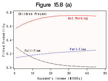
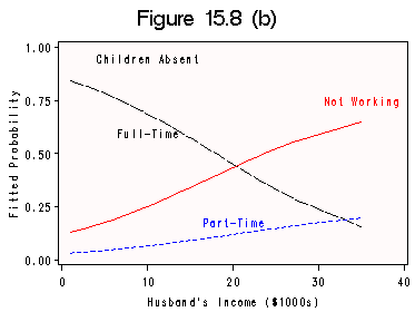
Calculation on page 468 and Figure 15.8 (a) and (b) on data file womenlf. We still use the same code scheme from last section.
proc catmod  data=wcoded;
  direct husbinc kid;/*to specify that they are continuous variables*/
  model w = husbinc kid / oneway noresponse;/*Can tell baseline from oneway table*/
  response out=catout;
run;

data catplot;
  set catout;
  array p(3);
  array q(3);
  if _type_ eq 'PROB' and kid=0 then
  p(_number_)=_pred_;
  if _type_ eq 'PROB' and kid=1 then
  q(_number_)=_pred_;
  keep p1 p2 p3 q1 q2 q3 husbinc;
  output;
run;

data lab1;
  length function style $ 8 text $17;
  retain function 'label' xsys  ysys '2' when 'a' color 'black';
  function='label'; x=10; y=0.78; size=1; color='black'; text='Children Present'; output;
  function='label'; x=35; y=0.72; size=1; color='red'; text='Not Working'; output;
  function='label'; x=35; y=.27; size=1; color='blue'; text='Part-Time'; output;
  function='label'; x=10; y=0.25; size=1; color='black'; text='Full-Time'; output;
run;

title 'Figure 15.8 (a)';
axis1 order=(0 to 50 by 10);
axis2 order=(0 to 0.8 by .2) label =(r=0 a =90);
symbol1 c=black v=none line=4 h=1 i=join;
symbol2 c=blue v=none line=2 h=1 i = join;
symbol3 c=red v=none line=1 h=1 i=join;
proc gplot data=catplot;
  plot q1*husbinc=1 q2*husbinc=2 q3*husbinc=3
  /annotate=lab1 overlay hminor=0 vminor=0 haxis=axis1 vaxis=axis2 cframe=snow;
  label husbinc='Husband''s Income ($1000s)';
  label q1='Fitted Probability';
  run;
quit;
data lab2;
  length function style $ 8 text $17;
  retain function 'label' xsys  ysys '2' when 'a' color 'black';
  function='label'; x=10; y=0.95; size=1; color='black'; text='Children Absent'; output;
  function='label'; x=35; y=0.75; size=1; color='red'; text='Not Working'; output;
  function='label'; x=20; y=.18; size=1; color='blue'; text='Part-Time'; output;
  function='label'; x=10; y=0.60; size=1; color='black'; text='Full-Time'; output;
run;

title 'Figure 15.8 (b)';
axis1 order=(0 to 40 by 10);
axis2 order=(0 to 1 by .25) label =(r=0 a =90);
symbol1 c=black v=none line=4 h=1 i=join;
symbol2 c=blue v=none line=2 h=1 i = join;
symbol3 c=red v=none line=1 h=1 i=join;
proc gplot data=catplot;
  plot p1*husbinc=1 p2*husbinc=2 p3*husbinc=3
  /annotate=lab2 haxis=axis1 vaxis=axis2 overlay hminor=0 vminor=0 cframe=snow;
  label husbinc='Husband''s Income ($1000s)';
  label p1='Fitted Probability';
  run;
quit;
The CATMOD Procedure
Response           w          Response Levels    3
Weight Variable    None       Populations       46
Data Set           WCODED     Total Frequency  263
Frequency Missing  0          Observations     263


     One-Way Frequencies

Variable    Value   Frequency
-----------------------------
w            0             66
             1             42
             2            155 <---This is the value for baseline.

(More output omitted here.)

            Maximum Likelihood Analysis

                Sub           -2 Log    Convergence
Iteration    Iteration    Likelihood      Criterion
---------------------------------------------------
     0           0         577.87006         1.0000
     1           0         430.05981         0.2558
     2           0         423.04966         0.0163
     3           0         422.88205       0.000396
     4           0         422.88193      2.9496E-7
     5           0         422.88193      4.418E-13

                              Maximum Likelihood Analysis

                                         Parameter Estimates
Iteration            1            2            3            4            5            6
---------------------------------------------------------------------------------------
     0               0            0            0            0            0            0
     1          1.6451      -0.5022      -0.0616      -0.0152      -2.5035      -0.8029
     2          1.8666      -1.3618      -0.0900     0.007921      -2.4978      -0.0311
     3          1.9801      -1.4285      -0.0971     0.006855      -2.5570       0.0185
     4          1.9828      -1.4323      -0.0972     0.006892      -2.5586       0.0215
     5          1.9828      -1.4323      -0.0972     0.006892      -2.5586       0.0215

           Maximum likelihood computations converged.
           Maximum Likelihood Analysis of Variance

Source               DF   Chi-Square    Pr > ChiSq
--------------------------------------------------
Intercept             2        29.35        <.0001
husbinc               2        12.82        0.0016
kid                   2        53.98        <.0001

Likelihood Ratio     86       138.67        0.0003


               Analysis of Maximum Likelihood Estimates

                                     Standard        Chi-
Effect       Parameter    Estimate      Error      Square    Pr > ChiSq
-----------------------------------------------------------------------
Intercept         1         1.9828     0.4842       16.77        <.0001
                  2        -1.4323     0.5925        5.84        0.0156
husbinc           3        -0.0972     0.0281       11.98        0.0005
                  4        0.00689     0.0235        0.09        0.7689
kid               5        -2.5586     0.3622       49.90        <.0001
                  6         0.0215     0.4690        0.00        0.9635
Calculation on nested dichotomies in subsection 15.2.2. Notice that in SAS proc logistic the option rsq on the model statement gives generalized R-sqaure, which is not the same as in the book. The second proc logistic below is for the purpose of computing (G0)2 at the bottom of the page using -2*Log L.
proc logistic data=wcoded; /* [15.27]*/
  model wstatus =husbinc kid/rsq;
  test husbinc; /*returns Wald test*/
  run;

proc logistic data=wcoded;
  model wstatus = kid /rsq;
  run;
The LOGISTIC Procedure ---[15.27]

(Most of the output is omitted here.)
         Model Fit Statistics

                              Intercept
               Intercept         and
Criterion        Only        Covariates
AIC              358.151        325.733
SC               361.723        336.449
-2 Log L         356.151        319.733 <--Needed for likelihood-ratio test


R-Square    0.1293    Max-rescaled R-Square    0.1743 <--generalized R-square

             Analysis of Maximum Likelihood Estimates

                               Standard
Parameter    DF    Estimate       Error    Chi-Square    Pr > ChiSq
Intercept     1      1.3358      0.3838       12.1164        0.0005
husbinc       1     -0.0423      0.0198        4.5750        0.0324
kid           1     -1.5756      0.2923       29.0650        <.0001

      Linear Hypotheses Testing Results  <-- Wald test on the effect of income

                   Wald
 Label       Chi-Square      DF    Pr > ChiSq
 Test 1          4.5750       1        0.0324
The LOGISTIC Procedure --for the likelihood-ratio test on the effect on income

(Most of the output is omitted here.)

         Model Fit Statistics

                              Intercept
               Intercept         and
Criterion        Only        Covariates
AIC              358.151        328.559
SC               361.723        335.703
-2 Log L         356.151        324.559 <--Needed for likelihood-ratio test

R-Square    0.1132    Max-rescaled R-Square    0.1526
data wcode1; /*full-time vs. part-time*/
  set womenlf;
  if (work='fulltime') then wstatus=1;
  else if (work = 'parttime') then wstatus=0;
  if (child ='present') then kid = 1;
  else kid =0;
  run;

proc logistic data=wcode1 descending;/*formula on p. 473: part-time vs. full-time*/
  model wstatus= husbinc kid /rsq;
The LOGISTIC Procedure --full-time vs. part-time

 (Most of the output omitted here.)

         Model Fit Statistics

                              Intercept
               Intercept         and
Criterion        Only        Covariates
AIC              146.342        110.495
SC               149.024        118.541
-2 Log L         144.342        104.495


R-Square    0.3085    Max-rescaled R-Square    0.4185
        Testing Global Null Hypothesis: BETA=0

Test                 Chi-Square       DF     Pr > ChiSq
Likelihood Ratio        39.8468        2         <.0001
Score                   35.1502        2         <.0001
Wald                    25.5820        2         <.0001

             Analysis of Maximum Likelihood Estimates

                               Standard
Parameter    DF    Estimate       Error    Chi-Square    Pr > ChiSq
Intercept     1      3.4778      0.7671       20.5536        <.0001
husbinc       1     -0.1073      0.0392        7.5062        0.0061
kid           1     -2.6514      0.5411       24.0134        <.0001
data wcode2;
  set womenlf;
  if (work='not_work') then  w=2;
  else if (work='fulltime') then w=0;
  else w=1;
  if (child ='present') then kid = 1;
  else kid =0;
  ik=husbinc*kid;
run;

proc logistic data=wcode2;
  model w=husbinc kid / rsq ;
  run;
The LOGISTIC Procedure

(Most of the output is omitted here.)

         Model Fit Statistics

                              Intercept
               Intercept         and
Criterion        Only        Covariates
 AIC              504.493        449.663
SC               511.637        463.952
-2 Log L         500.493        441.663


        Testing Global Null Hypothesis: BETA=0

Test                 Chi-Square       DF     Pr > ChiSq
Likelihood Ratio        58.8296        2         <.0001
Score                   54.6338        2         <.0001
Wald                    53.9013        2         <.0001

              Analysis of Maximum Likelihood Estimates

                                Standard
Parameter     DF    Estimate       Error    Chi-Square    Pr > ChiSq
Intercept      1      0.9409      0.3619        6.7579        0.0093
Intercept2     1      1.8520      0.3773       24.0994        <.0001
husbinc        1     -0.0539      0.0194        7.6913        0.0055
kid            1     -1.9719      0.2804       49.4637        <.0001
Section 15.3 Discrete Independent Variables and Contingency Tables
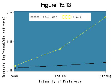
The analysis in this section is based on Table 15.3, which is based on data from an example from The American Voter (Campbell et al. 1960). The first dataset is created based on Table 15.3 for Figure 15.13.
data logvote;
  input   logv_one logv_close intensity;
  label   intensity ='0 for weak, 1 for medium and 2 for strong';
datalines;
.847 .9 0
.904 1.318 1
.981 2.084 2
;
run;
title 'Figure 15.13';
filename outfiles 'https://stats.idre.ucla.edu/wp-content/uploads/2016/02/chp15Fig13.gif';
axis1  label =(r=0 a=90) order=(0.8 to 2.2 by .7);
axis2 value=('Weak' 'Medium' 'Strong');
symbol1 c=black v=star i=join line=1 ;
symbol2 c=yellow v=circle i=join line=2;
legend1 label=none
        shape=symbol(4,2)
		cframe=white
        position=(top center inside)
		value=('One-sided' 'Close')
		mode=share;
proc gplot data=logvote;
  plot logv_one*intensity=1 logv_close*intensity=2 /
  overlay vaxis=axis1 haxis=axis2 vminor=0 hminor=0 lengend=lengend1 cframe=steel;
  label intensity='Intensity of Preference';
  label logv_one = 'Turnout: log(voted/did not vote)';
run;
quit;
In order to do the logistic regression, we create another dataset based on Table 15.3 again using the turnout frequencies as weight. For Table 15.4 and Table 15.5 we run proc logistic for each model and obtain (G0)2 by taking the difference of -2*Log L from each pair models being compared. Table 15.5 is produced in the last data step and proc print using SAS function probchi.
data election;
  input perclose inten1 inten2 voted wv;
  label perclose ='0 for one-sided 1 for close'
  intens1 ='baseline: weak'
  voted = '0 for not 1 for yes';
  clspref1=perclose*inten1;
  clspref2=perclose*inten2;
cards;
0 0 0 1 91
0 0 0 0 39
0 1 0 1 121
0 1 0 0 49
0 0 1 1 64
0 0 1 0 24
1 0 0 1 214
1 0 0 0 87
1 1 0 1 284
1 1 0 0 76
1 0 1 1 201
1 0 1 0 25
;
run;

proc logistic data=election; /*model 1*/
  model voted = perclose inten1 inten2 clspref1 clspref2;
  weight wv;
  test: test clspref1=0, clspref2=0;
run;
proc logistic data=election; /*model 2*/
  model voted = perclose inten1 inten2;
  weight wv;
run;

proc logistic data=election; /*model 3*/
  model voted = perclose clspref1 clspref2;
  weight wv;
run;

proc logistic data=election; /*model 4*/
  model voted = inten1 inten2 clspref1 clspref2;
  weight wv;
  run;

proc logistic data=election; /*model 5*/
  model voted = perclose;
  weight wv;
run;

proc logistic data=election; /*model 6*/
  model voted = inten1 inten2;
  weight wv;
run;
(Most of the output is omitted here.)

The LOGISTIC Procedure --Model 1--
         Model Fit Statistics

                              Intercept
               Intercept         and
Criterion        Only        Covariates

-2 Log L        1391.266       1356.434

The LOGISTIC Procedure --Model 2--
         Model Fit Statistics

                              Intercept
               Intercept         and
Criterion        Only        Covariates

-2 Log L        1391.266       1363.553

The LOGISTIC Procedure --Model 3--
         Model Fit Statistics

                              Intercept
               Intercept         and
Criterion        Only        Covariates

-2 Log L        1391.266       1356.625

The LOGISTIC Procedure --Model 4--
         Model Fit Statistics

                              Intercept
               Intercept         and
Criterion        Only        Covariates

-2 Log L        1391.266       1356.487

The LOGISTIC Procedure --Model 5--
         Model Fit Statistics

                              Intercept
               Intercept         and
Criterion        Only        Covariates

-2 Log L        1391.266       1382.658
The LOGISTIC Procedure --Model 6--
         Model Fit Statistics

                              Intercept
               Intercept         and
Criterion        Only        Covariates

-2 Log L        1391.266       1371.838
data logL;
  input  models $ df g1  g2  @g p;
  g=g1-g2;
  p=1-probchi(g1-g2,df);
drop g1 g2;
cards;
  6-2  1 1371.838 1363.552
  4-1  1 1356.487 1356.434
  5-2  2 1382.658 1363.552
  3-1  2 1356.625 1356.434
  2-1  2 1363.552 1356.434
;
run;
proc print data=logL;
run;
Obs    models    df       g         p
 1      6-2       1     8.286    0.00400
 2      4-1       1     0.053    0.81792
 3      5-2       2    19.106    0.00007
 4      3-1       2     0.191    0.90892
 5      2-1       2     7.118    0.02847

