In this chapter we will be using the hmohiv and the uis data sets.
Table 4.2, p. 119
Proportional hazard model containing only the predictor drug using the hmohiv data.
proc phreg data=hmohiv;
  model time*censor(0) = drug / rl;
run;

<output omitted>

                         Analysis of Maximum Likelihood Estimates

               Parameter    Standard                            Hazard   95% Hazard Ratio
Variable  DF    Estimate       Error  Chi-Square  Pr > ChiSq     Ratio   Confidence Limits
drug       1     0.77919     0.24226     10.3451      0.0013     2.180     1.356     3.504
Table 4.3, p. 121.
Creating the design variables for age.
data cat;
  set hmohiv;
  age2 = (age ge 30 & age le 34);
  age3 = (age ge 35 & age le 39);
  age4 = (age ge 40);
run;
Table 4.4 and 4.5, p. 122-123.
The coefficients and hazard ratio from the proportional hazard model which includes the design variables for age.
proc phreg data=cat;
  model time*censor(0) = age2 age3 age4 / rl;
run;

<output omitted>

                         Analysis of Maximum Likelihood Estimates

               Parameter    Standard                            Hazard   95% Hazard Ratio
Variable  DF    Estimate       Error  Chi-Square  Pr > ChiSq     Ratio   Confidence Limits
age2       1     1.19659     0.45099      7.0399      0.0080     3.309     1.367     8.009
age3       1     1.31293     0.45885      8.1873      0.0042     3.717     1.512     9.136
age4       1     1.86003     0.46926     15.7113      <.0001     6.424     2.561    16.115
Table 4.6, p. 125.
This is the same model as in table 4.4 and table 4.5, therefore, we don’t need to see the output again. This is why we use the noprint option. In order to obtain the variance-covariance matrix we use the covout option which will save the variance-covariance matrix in the data set specified by the outest option. We have chosen to call this data set temp. When we print, we only want to see the estimates for the predictors, so we look at the variables age2-age4 and _name_
proc phreg data=cat outest=temp covout noprint;
  model time*censor(0) = age2 age3 age4 / rl;
run;
proc print data=temp noobs;
 where _name_ ne 'time';
 var _name_ age2 age3 age4;
run;

<output omitted>

_NAME_      age2       age3       age4
 age2     0.20339    0.16361    0.17043
 age3     0.16361    0.21054    0.16657
 age4     0.17043    0.16657    0.22021
Testing if the oldest age group (age4) is different from the two middle age groups (age2 and age3), bottom of p. 125.
In order to do this in a regression model we must use the appropriate coding. For more information about contrast coding for regression models please refer to our web book on regression chapter 5.
data contrast;
  set cat;
  if age2=1 then agec = -1/3;
  if age3=1 then agec = -1/3;
  if age4=1 then agec = 2/3;
run;
proc phreg data=contrast;
  model time*censor(0) = agec ;
run;

<output omitted>

                     Analysis of Maximum Likelihood Estimates

                   Parameter      Standard                                  Hazard
Variable    DF      Estimate         Error    Chi-Square    Pr > ChiSq       Ratio
agec         1       0.60647       0.26134        5.3854        0.0203       1.834
Creating the design variables for age using deviation from mean coding, p. 126.
data contrast;
  set cat;
  if age le 29 then agenew2 = -1;
  else agenew2 = age2;
  if age le 29 then agenew3 = -1;
  else agenew3 = age3;
  if age le 29 then agenew4 = -1;
  else agenew4 = age4;
run;
Table 4.7, p. 127.
Proportional hazard model including the design variables for age using deviation from mean coding.
proc phreg data=contrast;
  model time*censor(0) = agenew2 agenew3 agenew4;
run;

<output omitted>

                     Analysis of Maximum Likelihood Estimates

                   Parameter      Standard                                  Hazard
Variable    DF      Estimate         Error    Chi-Square    Pr > ChiSq       Ratio
agenew2      1       0.10420       0.19205        0.2944        0.5874       1.110
agenew3      1       0.22054       0.20589        1.1475        0.2841       1.247
agenew4      1       0.76764       0.20931       13.4499        0.0002       2.155
Table 4.8, p. 129.
Proportional hazard model containing the predictor age.
proc phreg data=hmohiv;
  model time*censor(0) = age;
run;

<output omitted>

                     Analysis of Maximum Likelihood Estimates

                   Parameter      Standard                                  Hazard
Variable    DF      Estimate         Error    Chi-Square    Pr > ChiSq       Ratio
age          1       0.08141       0.01744       21.8006        <.0001       1.085
Creating the variable drug in the uis data set.
data uis;
  set uis;
  if ivhx ne . then drug = (ivhx ne 1);
run;
Table 4.9, p. 133.
Two proportional hazard models, one containing only drug and the other containing both drug and age. The where statement in the first model insures that both models use only the observation with complete data for both predictors.
proc phreg data=uis;
  where ivhx ne . and age ne . ;
  model time*censor(0) = drug;
run;

<output omitted>

Summary of the Number of Event and Censored Values

                                     Percent
   Total       Event    Censored    Censored
     605         489         116       19.17

                     Analysis of Maximum Likelihood Estimates

                   Parameter      Standard                                  Hazard
Variable    DF      Estimate         Error    Chi-Square    Pr > ChiSq       Ratio
drug         1       0.32099       0.09481       11.4623        0.0007       1.378

proc phreg data=uis;
  model time*censor(0) = drug age;
run;

<output omitted>

Summary of the Number of Event and Censored Values

                                     Percent
   Total       Event    Censored    Censored
     605         489         116       19.17

                     Analysis of Maximum Likelihood Estimates

                   Parameter      Standard                                  Hazard
Variable    DF      Estimate         Error    Chi-Square    Pr > ChiSq       Ratio
drug         1       0.43944       0.10072       19.0377        <.0001       1.552
age          1      -0.02638       0.00784       11.3236        0.0008       0.974
Table 4.10, p. 135.
Three proportional hazard models: the first containing only the predictor treat, the second containing both treat and age, and the third containing treat, age and the interaction of treat and age. The where statement in the first model insures that both models use only the observation with complete data for both predictors.
proc phreg data=uis;
  where treat ne . and age ne .;
  model time*censor(0) = treat;
run;

<output omitted>

Summary of the Number of Event and Censored Values

                                     Percent
   Total       Event    Censored    Censored
     623         504         119       19.10

                     Analysis of Maximum Likelihood Estimates

                   Parameter      Standard                                  Hazard
Variable    DF      Estimate         Error    Chi-Square    Pr > ChiSq       Ratio
treat        1      -0.21963       0.08932        6.0455        0.0139       0.803

proc phreg data=uis;
  model time*censor(0) = treat age;
run;

<output omitted>

Summary of the Number of Event and Censored Values

                                     Percent
   Total       Event    Censored    Censored
     623         504         119       19.10
                     Analysis of Maximum Likelihood Estimates

                   Parameter      Standard                                  Hazard
Variable    DF      Estimate         Error    Chi-Square    Pr > ChiSq       Ratio
treat        1      -0.22298       0.08933        6.2307        0.0126       0.800
age          1      -0.01327       0.00721        3.3847        0.0658       0.987

data interaction;
   set uis;
   agetreat = age*treat;
run;
proc phreg data=interaction;
  model time*censor(0) = treat age agetreat ;
run;

<output omitted>

Summary of the Number of Event and Censored Values

                                     Percent
   Total       Event    Censored    Censored
     623         504         119       19.10

                     Analysis of Maximum Likelihood Estimates

                   Parameter      Standard                                  Hazard
Variable    DF      Estimate         Error    Chi-Square    Pr > ChiSq       Ratio
treat        1       0.52188       0.47448        1.2098        0.2714       1.685
age          1      -0.00177       0.01013        0.0305        0.8613       0.998
agetreat     1      -0.02316       0.01450        2.5514        0.1102       0.977
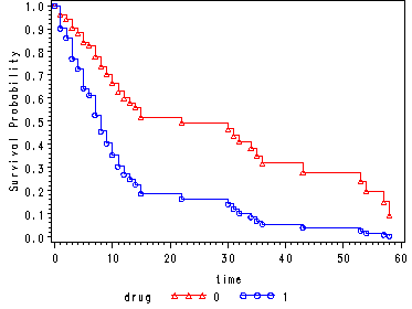
Fig. 4.2, p. 139.
Graph of the estimated proportional hazard model survivorship function for each drug group using the hmohiv data set. The curves here are “predicted” survival curves since each curve has 100 plotted values since the points are plotted at each observed time for both curves (refer to p. 142 for a more detailed explanation).
The first data step is used to artificially create a time point at time = 0 where the survival probability is equal to 1.
proc phreg data=hmohiv noprint;
  model time*censor(0) = drug ;
  output out=temp survival=survival;
run;
data temp;
  if _n_=1 then do;
  time = 0;
  survival = 1;
  end;
  output;
  set temp;
run;
data temp;
  set temp;
  if drug=0 or time = 0 then surv0 = survival;
  else surv0=. ;
  if drug=0 or time = 0 then surv1 = survival**exp(.779);
  else surv1=. ;
run;proc sort data=temp;
  by time drug;
run;
goptions reset=all;
symbol1 c=red v=triangle h=.8 i=stepjll;
symbol2 c=blue v=circle h=.8 i=stepjll;
legend1 label=none value=(height=1 font=swiss 'Drug=0' 'Drug=1' )
        position=(top right inside) mode=share cborder=black;
axis label=( a=90 'Survival Probability');
proc gplot data=temp;
  plot (surv0 surv1)*time / overlay legend=legend1 vaxis=axis1;
run;
quit;
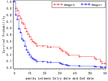
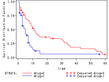
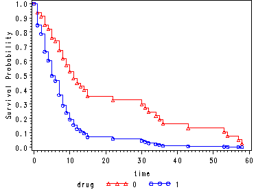
Fig. 4.3, p. 141.
Graph of the estimated proportional hazards survivorship function for each drug group using the hmohiv data set. Points are plotted at observed times for each curve.
goptions reset=all;
symbol1 c=red;
symbol2 c=blue;
proc lifetest data=hmohiv plots=(s);
  time time*censor(0);
  strata drug;
run;

<output omitted>
Creating the centered age variable, agec = age – 35.
data center;
  set hmohiv;
  agec = age - 35;
run;
Table 4.12, p. 143.
Proportional hazard model containing the predictors drug and agec.
proc phreg data=center ;
  model time*censor(0) = agec drug ;
run;

<output omitted>

                     Analysis of Maximum Likelihood Estimates

                   Parameter      Standard                                  Hazard
Variable    DF      Estimate         Error    Chi-Square    Pr > ChiSq       Ratio
agec         1       0.09151       0.01849       24.5009        <.0001       1.096
drug         1       0.94108       0.25550       13.5662        0.0002       2.563
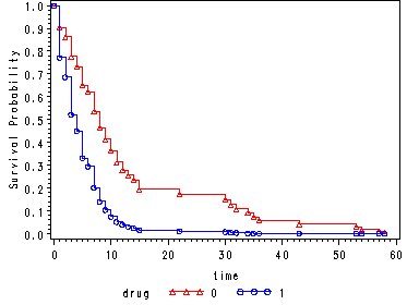
Fig. 4.4, p. 144.
data cov1;
  drug = 1;
  agec = 0;
run;
data hmohiv35;
  set hmohiv;
  agec = age - 35;
run;
proc phreg data=hmohiv35 noprint;
  model time*censor(0) = agec drug ;
  baseline out = temp1 survival=s covariates=cov1 /method=ch nomean;
run;
data hmohivd1;
  set hmohiv;
  where drug =1;
  keep time censor;
run;
proc sort data=hmohivd1;
  by time;
run;
data combo1;
  merge temp1 hmohivd1;
  by time;
run;
proc sort data = combo1;
  by time;
run;
data combo1;
  set combo1;
  by time;
  if censor = . and time ne 0 then delete;
  if first.time;
  if s = . then drug = 1;
  if s = . then s = 0;
run;
data cov0;
  drug = 0;
  agec = 0;
run;
proc phreg data=hmohiv35 noprint;
  model time*censor(0) = agec drug ;
  baseline out = temp0 survival=s covariates=cov0 /method=ch nomean;
run;
data hmohivd0;
  set hmohiv;
  where drug =0;
  keep time censor;
run;
proc sort data=hmohivd0;
  by time;
run;
data combo0;
  merge temp0 hmohivd0;
  by time;
run;
proc sort data=combo0;
  by time;
run;
data combo0;
  set combo0;
  if censor = . and time ne 0 then delete;
  by time;
  if first.time;
run;
data combo;
  set combo0 combo1;
  if drug ne . ;
run;
goptions reset=all;
symbol1 c=red v=triangle h=.8 i=stepjll;
symbol2 c=blue v=circle h=.8 i=stepjll;
axis1 label=(a=90 'Survival Probability');
proc gplot data = combo;
plot s*time = drug / vaxis=axis1;
run;
quit;
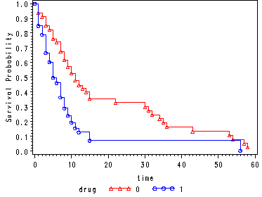
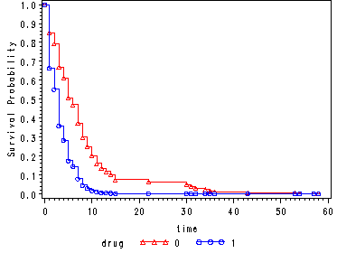
Fig. 4.5, p. 146.
Creating the covariate data sets.
data cov0;
  drug = 0;
  agec = 0;
  run;
data cov1;
  drug = 1;
  agec = 0;
run;
Creating the centered age variable, agec = age - 30.
data hmohiv30;
  set hmohiv;
  agec = age - 30;
run;
Generating the estimated survivorship function for drug=0 at agec=0 (the mean for agec) and for drug=1 at agec=0.
proc phreg data=hmohiv30 noprint;
  model time*censor(0) = agec drug ;
  baseline out = temp0 survival=s covariates=cov0 /method=ch nomean;
run;
proc phreg data=hmohiv30 noprint;
  model time*censor(0) = agec drug ;
  baseline out = temp1 survival=s covariates=cov1 /method=ch nomean;
run;
data combo;
  set temp0 temp1;
run;
goptions reset=all;
symbol1 c=red v=triangle h=.8 i=stepjll;
symbol2 c=blue v=circle h=.8 i=stepjll;
axis1 label=(a=90 'Survival Probability');
proc gplot data = combo;
  plot s*time=drug / vaxis = axis1;
run;
quit;
Creating the centered age variable, agec = age - 35.
Generating the estimated survivorship function for drug=0 at agec=0 (the mean for agec) and for drug=1 at agec=0.
data hmohiv35;
  set hmohiv;
  agec = age - 35;
run;
proc phreg data=hmohiv35 noprint;
  model time*censor(0) = agec drug ;
  baseline out = temp0 survival=s covariates=cov0 /method=ch nomean;
run;
proc phreg data=hmohiv35 noprint;
  model time*censor(0) = agec drug ;
  baseline out = temp1 survival=s covariates=cov1 /method=ch nomean;
run;
data combo;
  set temp0 temp1;
run;
goptions reset=all;
symbol1 c=red v=triangle h=.8 i=stepjll;
symbol2 c=blue v=circle h=.8 i=stepjll;
axis1 label=(a=90 'Survival Probability');
proc gplot data = combo;
  plot s*time=drug / vaxis=axis1;
run;
quit;
Creating the centered age variable, agec = age - 40.
Generating the estimated survivorship function for drug=0 at agec=0 (the mean for agec) and for drug=1 at agec=0.
data hmohiv40;
  set hmohiv;
  agec = age - 40;
run;
proc phreg data=hmohiv40 noprint;
  model time*censor(0) = agec drug ;
  baseline out = temp0 survival=s covariates=cov0 /method=ch nomean;
run;
proc phreg data=hmohiv40 noprint;
  model time*censor(0) = agec drug ;
  baseline out = temp1 survival=s covariates=cov1 /method=ch nomean;
run;
data combo;
  set temp0 temp1;
run;
goptions reset=all;
symbol1 c=red v=triangle h=.8 i=stepjll;
symbol2 c=blue v=circle h=.8 i=stepjll;
axis1 label=(a=90 'Survival Probability');
proc gplot data = combo;
  plot s*time=drug / vaxis=axis1;
run;
quit;
Creating the centered age variable, agec = age - 45.
Generating the estimated survivorship function for drug=0 at agec=0 (the mean for agec) and for drug=1 at agec=0.
data hmohiv45;
  set hmohiv;
  agec = age - 45;
run;

proc phreg data=hmohiv45 noprint;
  model time*censor(0) = agec drug ;
  baseline out = temp0 survival=s covariates=cov0 /method=ch nomean;
run;
proc phreg data=hmohiv45 noprint;
  model time*censor(0) = agec drug ;
  baseline out = temp1 survival=s covariates=cov1 /method=ch nomean;
run;
data combo;
   set temp0 temp1;
run;
goptions reset=all;
symbol1 c=red v=triangle h=.8 i=stepjll;
symbol2 c=blue v=circle h=.8 i=stepjll;
axis1 label=(a=90 'Survival Probability');
proc gplot data = combo;
  plot s*time=drug / vaxis=axis1;
run;
quit;
Creating the centered variable for age, agec = age - 30 and for ndrugtx, ndrugtx_c = ndrugtx - 3. The variable drug has already been created: drug = 0 when ivhx = 1 and drug = 1 otherwise.
data uis;
  set uis;
  agec = age - 30;
  ndrugtx_c = ndrugtx - 3;
run;
Table 4.13, p. 148.
Proportional hazard model containing the predictors treat, agec, drug and ndrugtx_c.
proc phreg data=uis;
  model time*censor(0) = treat agec drug  ndrugtx_c ;
run;

<output omitted>

                     Analysis of Maximum Likelihood Estimates

                    Parameter      Standard                                  Hazard
Variable     DF      Estimate         Error    Chi-Square    Pr > ChiSq       Ratio
treat         1      -0.22710       0.09158        6.1496        0.0131       0.797
agec          1      -0.03074       0.00794       15.0081        0.0001       0.970
drug          1       0.34258       0.10426       10.7960        0.0010       1.409
ndrugtx_c     1       0.03091       0.00799       14.9710        0.0001       1.031
Obtaining the means for the predictors in the previous model.
proc means data= uis mean;
  var drug ndrugtx_c;
run;

The MEANS Procedure

Variable             Mean
-------------------------
drug            0.6180328
ndrugtx_c       1.5744681
-------------------------
Creating the covariate data sets to be used in the baseline statement of proc phreg.
data cov0;
  treat = 0;
  drug = 0.6180328;
  agec = 0;
  ndrugtx_c =  1.5744681;
run;
data cov1;
  treat = 1;
  drug = 0.6180328;
  agec = 0;
  ndrugtx_c =  1.5744681;
run;
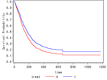
Obtaining the estimated survivorship function for both treatment groups. Then creating two extra observations in order to extend the curves in the graph to the last time point (time=1172) using the same covariate pattern as the prior time point (time=659).
proc phreg data=uis noprint;
  model time*censor(0) = treat agec drug  ndrugtx_c ;
  baseline out = temp0 survival=s covariates=cov0 /method=ch nomean;
run;
proc phreg data=uis noprint;
  model time*censor(0) = treat agec drug  ndrugtx_c ;
  baseline out = temp1 survival=s covariates=cov1 /method=ch nomean;
run;
data combo;
   set temp0 temp1;
run;
proc print data=combo noobs;
  where time > 600;
run;

                            ndrugtx_
treat    agec      drug         c       time       s
  0        0     0.61803     1.57447     659    0.10316
  1        0     0.61803     1.57447     659    0.16366

data combo;
  if _n_ = 1 then do;
  time = 1172.00;
  s= 0.10316;
  treat = 0;
  agec=0;
  drug =  0.61803;
  ndrugtx_c =  1.57447;
  end;
  if _n_ = 2 then do;
  time = 1172.00;
  s=  0.16366;
  treat = 1;
    agec=0;
  drug =  0.61803;
  ndrugtx_c =  1.57447;
  end;
  output;
  set combo;
run;
proc sort data=combo;
  by time;
run;
goptions reset=all;
symbol1 c=red v=none h=.8 i=stepjll;
symbol2 c=blue v=none h=.8 i=stepjll;
axis1 label=(a=90 'Survival Probability') order=(0 to 1.0 by .1);
proc gplot data = combo;
  plot s*time=treat / vaxis=axis1;
run;
quit;