Page 245 Table 11.1 Means and standard deviations for nondepressed and depressed adults in Los Angeles County
data depress;
set "c:\cama3\depress";
run;

proc sort data = depress out=depress;
by cases;
run;

proc means data = depress mean std;
var sex age educat income health beddays acuteill chronill;
by cases;
run;
CASES=0

The MEANS Procedure

Variable            Mean         Std Dev
----------------------------------------
SEX            1.5860656       0.4935494
AGE           45.2418033      18.1464928
EDUCAT         3.5450820       1.3310228
INCOME        21.6762295      15.9754727
HEALTH         1.7131148       0.7958690
BEDDAYS        0.1721311       0.3782703
ACUTEILL       0.2786885       0.4492755
CHRONILL       0.4836066       0.5007584
----------------------------------------

CASES=1

Variable            Mean         Std Dev
----------------------------------------
SEX            1.8000000       0.4040610
AGE           40.3800000      17.4003167
EDUCAT         3.1600000       1.1668902
INCOME        15.2000000       9.8374545
HEALTH         2.0600000       0.9775020
BEDDAYS        0.4200000       0.4985694
ACUTEILL       0.3800000       0.4903144
CHRONILL       0.6200000       0.4903144
----------------------------------------
Page 248 Figure 11.2 Distribution of income for depressed and nondepressed individuals showing effects of a dividing point at an income of $18440.
We were unable to reproduce this graph.
Page 249 Table 11.2 Classification of individuals as depressed or not depressed on the basis of income alone.
proc discrim data = depress;
class cases;
var income;
run;
<some output omitted>
Number of Observations and Percent Classified into CASES

  From
 CASES            0            1        Total

     0          121          123          244
              49.59        50.41       100.00

     1           19           31           50
              38.00        62.00       100.00

 Total          140          154          294
              47.62        52.38       100.00
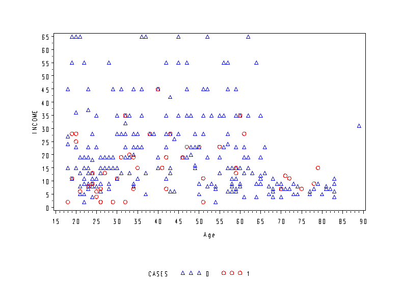
Page 252 Figure 11.5 Classification of individuals as depressed or not depressed on the basis of income and age.
NOTE: The line can be added using an annotated data set.
goptions reset = all;
goptions cells;
axis1 order=(0 to 65 by 5) label=('Income') label=(a=90 r = 0);
axis2 order=(15 to 90 by 5) label=('Age');
symbol1  v=triangle height=1 cells c=blue;
symbol2  v=circle height=1 cells c=red;
proc gplot data=depress ;
plot income*age = cases /vaxis = axis1 haxis = axis2;
run;
quit;
Page 253 Table 11.3 Classification of individuals as depressed or not depressed on the basis of income and age
proc discrim data = depress;
class cases;
var income age;
run;
<some output omitted>
Number of Observations and Percent Classified into CASES

  From
 CASES            0            1        Total

     0          154           90          244
              63.11        36.89       100.00

     1           20           30           50
              40.00        60.00       100.00

 Total          174          120          294
              59.18        40.82       100.00
Page 257 Table 11.4 Classification function and discriminant coefficients for age and income from BMDP 7M
NOTE: We do not know why the constant is incorrect.
NOTE: We do not know how to get the discriminant functions.
proc discrim data = depress;
class cases;
var age income;
run;
<some output omitted>
Linear Discriminant Function for CASES

Variable             0             1

Constant      -5.17094      -3.65520
AGE            0.16342       0.14249
INCOME         0.13603       0.10242
Page 258 Covariances in the middle of the page
proc corr data = depress cov;
var age income;
run;
The CORR Procedure

   2  Variables:    AGE      INCOME


       Covariance Matrix, DF = 293

                     AGE            INCOME

AGE          327.0831882       -53.0072671
INCOME       -53.0072671       233.7878967
<some output omitted>
Page 268 Table 11.5 Partial printout from BMDP 7M for classification into more than two groups, using the depression data with K = 3 groups
NOTE: Before you can do this, you need to add a new variable to the data set and use the variable cesd to recode the new variable, which we called cases3.
NOTE: The signs of the coefficients for canonical variables is arbitrary. The signs of the canonical variables given by SAS is opposite to what is shown in the text.
data depress1;
set depress;
if cesd = 0 then cases3 = 1;
if cesd ge 1 and cesd le 15 then cases3 = 2;
if cesd ge 16 then cases3 = 3;
run;

proc discrim data = depress1 can out=candepress;
class cases3;
var sex age educat income health beddays;
run;
<some output omitted>
The DISCRIM Procedure

Linear Discriminant Function

               _     -1 _                              -1 _
Constant = -.5 X' COV   X      Coefficient Vector = COV   X
                j        j                                 j


     Linear Discriminant Function for cases3

Variable             1             2             3

Constant     -16.52247     -17.44950     -17.71770
SEX            7.07529       7.49617       8.14165
AGE            0.16774       0.13935       0.11698
EDUCAT         2.54993       2.82551       2.68116
INCOME         0.10533       0.09005       0.06537
HEALTH         2.13954       2.75024       3.10425
BEDDAYS       -0.97394      -0.80246       0.46685

         Raw Canonical Coefficients

Variable              Can1              Can2

SEX            0.731029500       0.019771251
AGE           -0.031672485      -0.025305150
EDUCAT         0.006170102       0.654808658
INCOME        -0.027576962       0.000673965
HEALTH         0.575237409       0.688216467
BEDDAYS        1.136441447      -1.131166668
Page 271 Figure 11.6 Plot of the canonical variables for the depression data set with k = 3 groups
We were unable to reproduce this graph.

