Page 252 Table 11.1 Means and standard deviations for nondepressed and depressed adults in Los Angeles County
data depress;
set "c:\cama4\depress";
run;

proc sort data = depress out=depress;
by cases;
run;

proc means data = depress mean std;
var sex age educat income health beddays acuteill chronill;
by cases;
run;
CASES=0

The MEANS Procedure

Variable            Mean         Std Dev
----------------------------------------
SEX            1.5860656       0.4935494
AGE           45.2418033      18.1464928
EDUCAT         3.5450820       1.3310228
INCOME        21.6762295      15.9754727
HEALTH         1.7131148       0.7958690
BEDDAYS        0.1721311       0.3782703
ACUTEILL       0.2786885       0.4492755
CHRONILL       0.4836066       0.5007584
----------------------------------------

CASES=1

Variable            Mean         Std Dev
----------------------------------------
SEX            1.8000000       0.4040610
AGE           40.3800000      17.4003167
EDUCAT         3.1600000       1.1668902
INCOME        15.2000000       9.8374545
HEALTH         2.0600000       0.9775020
BEDDAYS        0.4200000       0.4985694
ACUTEILL       0.3800000       0.4903144
CHRONILL       0.6200000       0.4903144
----------------------------------------
Page 254 Figure 11.2 Distribution of income for depressed and nondepressed individuals showing effects of a dividing point at an income of $18440.
NOTE: We were unable to reproduce this graph.
Page 255 Table 11.2 Classification of individuals as depressed or not depressed on the basis of income alone.
proc discrim data = depress;
class cases;
var income;
run;
<some output omitted>
Number of Observations and Percent Classified into CASES

  From
 CASES            0            1        Total

     0          121          123          244
              49.59        50.41       100.00

     1           19           31           50
              38.00        62.00       100.00

 Total          140          154          294
              47.62        52.38       100.00
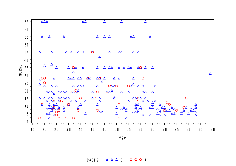
Page 258 Figure 11.5 Classification of individuals as depressed or not depressed on the basis of income and age.
NOTE: The line can be added using an annotated data set.
goptions reset = all;
goptions cells;
axis1 order=(0 to 65 by 5) label=('Income') label=(a=90 r = 0);
axis2 order=(15 to 90 by 5) label=('Age');
symbol1  v=triangle height=1 cells c=blue;
symbol2  v=circle height=1 cells c=red;
proc gplot data=depress ;
plot income*age = cases /vaxis = axis1 haxis = axis2;
run;
quit;

Page 259 Table 11.3 Classification of individuals as depressed or not depressed on the basis of income and age
proc discrim data = depress;
class cases;
var income age;
run;
<some output omitted>
Number of Observations and Percent Classified into CASES

  From
 CASES            0            1        Total

     0          154           90          244
              63.11        36.89       100.00

     1           20           30           50
              40.00        60.00       100.00

 Total          174          120          294
              59.18        40.82       100.00
Page 263 Table 11.4 Classification function and discriminant coefficients for age and income
NOTE: We do not know why the constant is incorrect.
NOTE: We do not know how to get the discriminant functions.
proc discrim data = depress;
class cases;
var age income;
run;
<some output omitted>
Linear Discriminant Function for CASES

Variable             0             1

Constant      -5.17094      -3.65520
AGE            0.16342       0.14249
INCOME         0.13603       0.10242
Page 263 Covariances at the bottom of the page
proc corr data = depress cov;
var age income;
run;
The CORR Procedure

   2  Variables:    AGE      INCOME


       Covariance Matrix, DF = 293

                     AGE            INCOME

AGE          327.0831882       -53.0072671
INCOME       -53.0072671       233.7878967
<some output omitted>
Page 270 middle of the page
NOTE: We have omitted most of the output from the proc discrim. The F test is produced by the manova option on the proc discrim statement.
proc discrim data = depress manova;
class cases;
var income age;
run;
<some output omitted>
The DISCRIM Procedure
Multivariate Statistics and Exact F Statistics
S=1 M=0 N=144.5
Statistic Value F Value Num DF Den DF Pr > F
Wilks' Lambda               0.95657959       6.60         2       291    0.0016
Pillai's Trace              0.04342041       6.60         2       291    0.0016
Hotelling-Lawley Trace      0.04539132       6.60         2       291    0.0016
Roy's Greatest Root         0.04539132       6.60         2       291    0.0016
Page 271 top of the page
NOTE: This F test is comparing two models. Hence we need to run proc discrim twice to get the numbers that we need. We have included only the relevant output below.
proc discrim data = depress;
class cases;
var income;
run;
The DISCRIM Procedure
Observations     294          DF Total               293
Variables          1          DF Within Classes      292
Classes            2          DF Between Classes       1
Class Level Information
          Variable                                                  Prior
 cases    Name        Frequency       Weight    Proportion    Probability
     0    _0                244     244.0000      0.829932       0.500000
     1    _1                 50      50.0000      0.170068       0.500000
Generalized Squared Distance to cases
  From
 cases             0             1
     0             0       0.18345
     1       0.18345             0
proc discrim data = depress;
class cases;
var income age;
run;
The DISCRIM Procedure
Observations     294          DF Total               293
Variables          2          DF Within Classes      292
Classes            2          DF Between Classes       1
Class Level Information
          Variable                                                  Prior
 cases    Name        Frequency       Weight    Proportion    Probability
     0    _0                244     244.0000      0.829932       0.500000
     1    _1                 50      50.0000      0.170068       0.500000
Generalized Squared Distance to cases
  From
 cases             0             1
     0             0       0.31941
     1       0.31941             0
