Page 341 Table 13.2 Kaplan-Meier estimates for data from Figure 13.2
data temp;
input id years dead;
cards;
1 2 1
2 6 1
3 2 0
4 3 0
5 1 1
;
run;
ods select ProductLimitEstimates;
proc lifetest data = temp;
time years*dead(0);
run;
quit;
The LIFETEST Procedure
Product-Limit Survival Estimates
                                     Survival
                                     Standard     Number      Number
   years     Survival    Failure      Error       Failed       Left
 0.00000       1.0000           0           0       0           5
 1.00000       0.8000      0.2000      0.1789       1           4
 2.00000       0.6000      0.4000      0.2191       2           3
 2.00000*           .           .           .       2           2
 3.00000*           .           .           .       2           1
 6.00000            0      1.0000           0       3           0
NOTE: The marked survival times are censored observations.
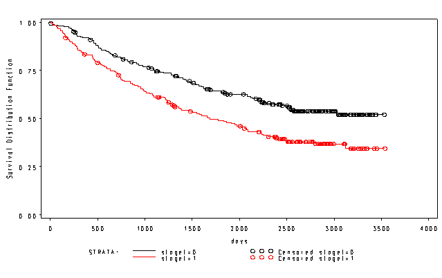
Page 342 Figure 13.6 Kaplan-Meier estimates of the survival functions for lung cancer data
NOTE: You cannot specify a path name on the proc lifetest statement; hence, we have created a temporary data set that is identical to the permanent one and used that.
data surv;
set 'd:surv';
run;
proc lifetest data = surv plots=(s) method=km;
time days*death(0);
strata staget;
run;

Page 347 Table 13.3 Percentage of deaths versus explanatory variables
data surv;
set "c:cama4surv";
run;

proc freq data = surv;
tables death*(staget perfbl treat poinf) / nopercent nofreq norow;
run;
The FREQ Procedure

Table of DEATH by POINF

DEATH     POINF

Col Pct |       0|       1|  Total
--------+--------+--------+
      0 |  50.26 |  25.00 |
--------+--------+--------+
      1 |  49.74 |  75.00 |
--------+--------+--------+
Total        380       20      400

Frequency Missing = 1
Page 348 Table 13.4 Log-linear model for lung cancer data: results
NOTE: The intercept given in the output is slightly different from that shown in the text. We suspect that the difference is caused by a change in the algorithms used in the different versions of SAS (an earlier version of SAS was used to generate the output shown in the text).
proc lifereg data = surv;
model days*death(0) = staget perfbl treat poinf /d=weibull;
run;
The LIFEREG Procedure

           Model Information

Data Set                       WORK.SURV
Dependent Variable             Log(DAYS)
Censoring Variable                 DEATH
Censoring Value(s)                     0
Number of Observations               398
Noncensored Values                   203
Right Censored Values                195
Left Censored Values                   0
Interval Censored Values               0
Missing Values                         3
Name of Distribution             Weibull
Log Likelihood              -512.7478113

Algorithm converged.

       Type III Analysis of Effects

                         Wald
Effect       DF    Chi-Square    Pr > ChiSq

STAGET        1       13.9320        0.0002
PERFBL        1        8.7069        0.0032
TREAT         1        0.2891        0.5908
POINF         1        5.3193        0.0211

                    Analysis of Parameter Estimates

                          Standard   95% Confidence     Chi-
Parameter     DF Estimate    Error       Limits       Square Pr > ChiSq

Intercept      1   8.6423   0.1584   8.3319   8.9527 2977.08     <.0001
STAGET         1  -0.5874   0.1574  -0.8959  -0.2790   13.93     0.0002
PERFBL         1  -0.5986   0.2029  -0.9963  -0.2010    8.71     0.0032
TREAT          1  -0.0831   0.1546  -0.3860   0.2198    0.29     0.5908
POINF          1  -0.7124   0.3089  -1.3178  -0.1070    5.32     0.0211
Scale          1   1.0894   0.0679   0.9641   1.2309
Weibull Shape  1   0.9180   0.0572   0.8124   1.0373
Page 349 Table 13.5 Cox’s model for lung cancer data: results
proc phreg data = surv;
model days*death(0) = staget perfbl treat poinf;
run;
The PHREG Procedure

                     Analysis of Maximum Likelihood Estimates

                   Parameter      Standard                                  Hazard
Variable    DF      Estimate         Error    Chi-Square    Pr > ChiSq       Ratio

STAGET       1       0.53654       0.14211       14.2542        0.0002       1.710
PERFBL       1       0.53080       0.18524        8.2110        0.0042       1.700
TREAT        1       0.07036       0.14182        0.2461        0.6198       1.073
POINF        1       0.66690       0.28040        5.6566        0.0174       1.948
We have skipped the examples on pages 350-354 because they use a simulated data set.
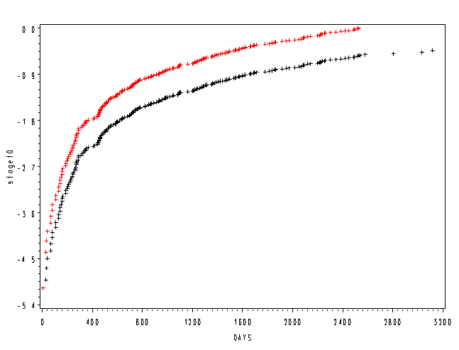
Page 357 Figure 13.9 Computer-generated graph of log(-logS(t)) versus t for lung cancer data (A = large tumor, B = small tumor)
data cov;
staget = 0;
perfbl = .1553885;
treat = .5137157;
poinf = .050;
run;

proc phreg data = surv;
model days*death(0) = staget perfbl treat poinf;
baseline covariates=cov loglogs=staget0 out=out0 / nomean;
run;

data cov1;
staget = 1;
perfbl = .1553885;
treat = .5137157;
poinf = .050;
run;

proc phreg data = surv;
model days*death(0) = staget perfbl treat poinf;
baseline covariates=cov1 loglogs=staget1 out=out1 / nomean;
run;

data fig138;
merge out0 out1;
by days;
run;

axis1 order=(0 to 3200 by 400);
axis2 order=(-5.4 to 0 by .9) label=(a=90);
proc gplot data = fig138;
plot (staget0 staget1)*days / overlay haxis=axis1 vaxis=axis2;
run;
quit;

