8.1 Logit Models for Nominal Responses
8.1.2 Alligator Food Choice Example
data gator;
input length choice $ @@;
cards;
1.24 I  1.30 I  1.30 I  1.32 F  1.32 F  1.40 F  1.42 I  1.42 F
1.45 I  1.45 O  1.47 I  1.47 F  1.50 I  1.52 I  1.55 I  1.60 I
1.63 I  1.65 O  1.65 I  1.65 F  1.65 F  1.68 F  1.70 I  1.73 O
1.78 I  1.78 I  1.78 O  1.80 I  1.80 F  1.85 F  1.88 I  1.93 I
1.98 I  2.03 F  2.03 F  2.16 F  2.26 F  2.31 F  2.31 F  2.36 F
2.36 F  2.39 F  2.41 F  2.44 F  2.46 F  2.56 O  2.67 F  2.72 I
2.79 F  2.84 F  3.25 O  3.28 O  3.33 F  3.56 F  3.58 F  3.66 F
3.68 O  3.71 F  3.89 F
;
run;
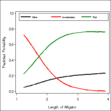
Table 8.2 on parameter estimates and Figure 8.1. Proc logistic of SAS 8.2 handles generalized logits model very nicely. The option link=glogit specifies that the model is generalized logit model. The option aggregate in the model statement requests a test on the global effect of variable length. In order to produce Figure 8.1, we need to generate predicted probabilities. This is accomplished by using output statement. Figure 8.1 is created using proc gplot.
proc logistic data=gator descending ;
  model choice (REFERENCE="O") = length / link=glogit scale=none aggregate;
  output out = prob PREDPROBS=I;
run;
axis1 label=(a = 90 "Predicted Probability") order = (0 to 1 by .2) minor=none;
axis2 label=("Length of Alligator") order = (1 to 4 by 1) minor = none;
legend1 label=none value=(h=2 font=swiss 'Other' 'Invertebrates' 'Fish')
       position=(top right inside) mode=share cborder=black;
symbol i = join w=2;
proc gplot data = prob;
  plot (ip_o ip_i ip_f)*length /overlay vaxis=axis1 haxis=axis2 legend=legend1;
run;
quit;
The LOGISTIC Procedure

               Model Information

Data Set                      WORK.GATOR
Response Variable             choice
Number of Response Levels     3
Number of Observations        59
Model                         generalized logit
Optimization Technique        Fisher's scoring

          Response Profile

 Ordered                      Total
   Value     choice       Frequency

       1     O                    8
       2     I                   20
       3     F                   31

Logits modeled use choice='O' as the reference category.

                    Model Convergence Status

         Convergence criterion (GCONV=1E-8) satisfied.

       Deviance and Pearson Goodness-of-Fit Statistics

Criterion        DF          Value     Value/DF     Pr > ChiSq

Deviance         86        75.1140       0.8734         0.7929
Pearson          86        80.1879       0.9324         0.6563

Number of unique profiles: 45

         Model Fit Statistics

                              Intercept
               Intercept         and
Criterion        Only        Covariates

AIC              119.142        106.341
SC               123.297        114.651
-2 Log L         115.142         98.341

        Testing Global Null Hypothesis: BETA=0

Test                 Chi-Square       DF     Pr > ChiSq

Likelihood Ratio        16.8006        2         0.0002
Score                   12.5702        2         0.0019
Wald                     8.9360        2         0.0115

       Type III Analysis of Effects

                        Wald
Effect      DF    Chi-Square    Pr > ChiSq

length       2        8.9360        0.0115

                  Analysis of Maximum Likelihood Estimates

                                         Standard          Wald
Parameter    choice    DF    Estimate       Error    Chi-Square    Pr > ChiSq

Intercept    I          1      5.6974      1.7938       10.0881        0.0015
Intercept    F          1      1.6177      1.3073        1.5314        0.2159
length       I          1     -2.4654      0.8997        7.5101        0.0061
length       F          1     -0.1101      0.5171        0.0453        0.8314

                 Odds Ratio Estimates

                         Point          95% Wald
Effect    choice      Estimate      Confidence Limits

length    I              0.085       0.015       0.496
length    F              0.896       0.325       2.468
Notice that the same parameter estimates can also be obtained by using proc catmod. We show the code here.
proc catmod data=gator;
  response logits;
  direct length;
  model choice = length ;
run;
quit;
8.1.4 Belief in Afterlife Example
data afterlife;
  input race gender belief count;
datalines;
1 1 1 371
1 1 2 49
1 1 3 74
1 0 1 250
1 0 2 45
1 0 3 71
0 1 1 64
0 1 2 9
0 1 3 15
0 0 1 25
0 0 2 5
0 0 3 13
;
run;
Table 8.4, Table 8.5 and Table 8.3. After generating the probabilities, we then generate the predicted counts. That is why Table 8.3 comes last.
proc logistic data = afterlife descending;
  weight count;
  model belief (reference="3") = race gender /link=glogit scale = none aggregate;
  output out = prob PREDPROBS=I;
run;

The LOGISTIC Procedure

       Type III Analysis of Effects

                        Wald
Effect      DF    Chi-Square    Pr > ChiSq

race         2        2.0824        0.3530
gender       2        7.2074        0.0272

                  Analysis of Maximum Likelihood Estimates

                                         Standard          Wald
Parameter    belief    DF    Estimate       Error    Chi-Square    Pr > ChiSq

Intercept    2          1     -0.7582      0.3614        4.4031        0.0359
Intercept    1          1      0.8828      0.2426       13.2390        0.0003
race         2          1      0.2712      0.3541        0.5863        0.4438
race         1          1      0.3420      0.2370        2.0814        0.1491
gender       2          1      0.1051      0.2465        0.1817        0.6699
gender       1          1      0.4186      0.1713        5.9737        0.0145
proc freq data = prob ;
format ip_1-ip_3 f4.2;
weight count;
tables race*gender*ip_1*ip_2*ip_3/list nocum nopercent out=test ;
run;
The FREQ Procedure

race    gender    IP_1    IP_2    IP_3    Frequency
---------------------------------------------------
   0         0    0.62    0.12    0.26          43
   0         1    0.71    0.10    0.19          88
   1         0    0.68    0.12    0.20         366
   1         1    0.75    0.10    0.15         494
data table8_3;
  set test;
  array p(3) ip_1-ip_3;
  array pre_count(3);
  do i = 1 to 3;
	 pre_count(i) = count*p(i);
	 end;
  drop ip_1-ip_3 i percent;
run;
proc print data = table8_3 noobs;
run;
                             pre_       pre_       pre_
race    gender    COUNT     count1     count2     count3

  0        0        43      26.752     5.1837    11.0648
  0        1        88      62.244     8.7615    16.9401
  1        0       366     248.245    44.1218    72.9396
  1        1       494     372.751    49.1838    72.064
8.2 Cumulative Logit Models for Ordinal Responses
8.2.2 Political Ideology Example
Table 8.6 and parameter estimates.
data ideology;
input party ideology count @@;
cards;
1 1 80   1 2 81   1 3 171   1 4 41   1 5 55
0 1 30   0 2 46   0 3 148   0 4 84   0 5 99
;
proc logistic data = ideology order=data descending;
  class party /param = ref;
  freq count;
  model ideology = party /link=clogit scale=none ;
  output out = prob PREDPROBS=I;
run;
proc freq data = prob noprint;
  weight count;
  tables party*ip_1*ip_2*ip_3*ip_4*ip_5
         /list nocum nopercent out=test ;
run;
data table8_6;
  set test;
  array p(5) ip_1-ip_5;
  array pcount(5);
  do i = 1 to 5;
	 pcount(i) = count*p(i);
	 end;
  drop ip_1-ip_5 i percent;
run;
proc print data = table8_6 noobs;
run;
           Testing Global Null Hypothesis: BETA=0

Test                 Chi-Square       DF     Pr > ChiSq

Likelihood Ratio        58.6451        1         <.0001
Score                   57.2448        1         <.0001
Wald                    57.0182        1         <.0001

           Type III Analysis of Effects

                        Wald
Effect      DF    Chi-Square    Pr > ChiSq

party        1       57.0182        <.0001

	   Analysis of Maximum Likelihood Estimates

                                 Standard          Wald
Parameter      DF    Estimate       Error    Chi-Square    Pr > ChiSq

Intercept 5     1     -2.0440      0.1188      295.9293        <.0001
Intercept 4     1     -1.2116      0.1031      138.0265        <.0001
Intercept 3     1      0.5000      0.0943       28.1405        <.0001
Intercept 2     1      1.4945      0.1134      173.6781        <.0001
party     0     1      0.9745      0.1291       57.0182        <.0001

    Odds Ratio Estimates

                   Point          95% Wald
Effect          Estimate      Confidence Limits

party 0 vs 1       2.650       2.058       3.412


party    COUNT    pcount1    pcount2    pcount3    pcount4    pcount5

  0       407     31.7714    44.0346    151.708    75.5005    103.985
  1       428     78.4308    83.1523    168.226    49.1170     49.074
8.2.3 Invariance to Choice of Response Categories
8.2.2 Political Ideology Example
Result in this section.
data ideology1;
  set ideology;
  if ideology = 1 or ideology = 2 then ideo = 1;
  else if ideology = 4 or ideology = 5 then ideo = 3;
  else ideo = 2;
run;

proc logistic data = ideology1 order=data descending;
  class party /param = ref;
  freq count;
  model ideo = party /link=clogit scale=none ;
run;
The LOGISTIC Procedure

         Model Fit Statistics

                              Intercept
               Intercept         and
Criterion        Only        Covariates

AIC             1826.542       1768.834
SC              1835.997       1783.016
-2 Log L        1822.542       1762.834

        Testing Global Null Hypothesis: BETA=0

Test                 Chi-Square       DF     Pr > ChiSq

Likelihood Ratio        59.7085        1         <.0001
Score                   58.5204        1         <.0001
Wald                    57.9280        1         <.0001

       Type III Analysis of Effects

                        Wald
Effect      DF    Chi-Square    Pr > ChiSq

party        1       57.9280        <.0001

              Analysis of Maximum Likelihood Estimates

                                 Standard          Wald
Parameter      DF    Estimate       Error    Chi-Square    Pr > ChiSq

Intercept 3     1     -1.2195      0.1041      137.1879        <.0001
Intercept 2     1      0.4931      0.0951       26.8774        <.0001
party     0     1      1.0059      0.1322       57.9280        <.0001
8.3 Paired-Category Logits for Ordinal Responses
8.3.2 Political Ideology Example Revisited
SAS proc catmod is the procedure to use for adjacent-categories logit models. Here is the syntax for a general adjacent-categories logit model. The response statement below specifies that the model is adjacent-categories logit model.
proc catmod data = ideology;
  weight count;
  response alogits;
  model ideology = party;
run;
quit;
The syntax for the simpler adjacent-categories model (8.3.2) on page 216 is slightly different. Here is a simple way of doing it. The _RESPONSE_ keyword allows modeling the levels of ideology. The coding for variable party uses simple coding scheme.
proc catmod data = ideology;
 weight count;
 response alogits;
 model ideology = _response_ party ;
 run;
quit;
If we want to dummy code the variable party, we can specify the design matrix directly as in the following example. Notice the sign difference of parameter estimate for variable party from the book on page 217. This is because our party is coded in the opposite way from the book.
proc catmod data = ideology ;
  weight count;
  population party;
  response alogits;
  model ideology = (1 0 0 0 0,
                    0 1 0 0 0,
                    0 0 1 0 0,
                    0 0 0 1 0,
		    1 0 0 0 1,
		    0 1 0 0 1,
	            0 0 1 0 1,
	            0 0 0 1 1)
	        (1='Group2/1', 2='Group3/2', 3='Group4/3', 4='Group5/4', 5='party');
run;
quit;
The CATMOD Procedure
                    Data Summary

Response           ideology     Response Levels    5
Weight Variable    count        Populations        2
Data Set           IDEOLOGY     Total Frequency  835
Frequency Missing  0            Observations      10

     Population Profiles

Sample    party    Sample Size
------------------------------
    1     0                407
    2     1                428

 Response Profiles

Response    ideology
--------------------
    1       1
    2       2
    3       3
    4       4
    5       5

                    Response Functions and Design Matrix

          Function      Response                  Design Matrix
Sample     Number       Function        1        2        3        4        5
-----------------------------------------------------------------------------
    1          1         0.42744        1        0        0        0        0
               2         1.16857        0        1        0        0        0
               3        -0.56640        0        0        1        0        0
               4         0.16430        0        0        0        1        0

    2          1         0.01242        1        0        0        0        1
               2         0.74721        0        1        0        0        1
               3        -1.42809        0        0        1        0        1
               4         0.29376        0        0        0        1        1

           Analysis of Variance

Source       DF   Chi-Square    Pr > ChiSq
------------------------------------------
Group2/1      1         9.82        0.0017
Group3/2      1       109.13        <.0001
Group4/3      1        43.44        <.0001
Group5/4      1         8.32        0.0039
party         1        52.63        <.0001

Residual      3         5.38        0.1459


            Analysis of Weighted Least Squares Estimates

                                  Standard        Chi-
Effect    Parameter    Estimate      Error      Square    Pr > ChiSq
--------------------------------------------------------------------
Model          1         0.4368     0.1394        9.82        0.0017
               2         1.1710     0.1121      109.13        <.0001
               3        -0.7161     0.1087       43.44        <.0001
               4         0.3534     0.1225        8.32        0.0039
               5        -0.4318     0.0595       52.63        <.0001
8.3.4 Continuation-Ratio Logits
We will use proc catmod in this section. In proc catmod, we can specify the response function using the response statement. Also, we need to pad empty cells in order for proc catmod to perform the parameter estimation successfully. This can be done using option addcell in the model statement.
data toxicity;
input con r count;
cards;
0 1 15
0 2 1
0 3 281
62.5 1 17
62.5 2 0
62.5 3 225
125 1 22
125 2 7
125 3 283
250 1 38
250 2 59
250 3 202
500 1 144
500 2 132
500 3 9
;
run;
proc catmod data = toxicity;
  weight count;
  direct con;
  response  0   1  -1,
            1 -.5 -.5 log;
  model r = con /addcell=.0005;
run;
quit;

The CATMOD Procedure

           Analysis of Weighted Least Squares Estimates

          Function               Standard        Chi-
Parameter  Number     Estimate      Error      Square    Pr > ChiSq
-------------------------------------------------------------------
Intercept    1         -4.4392     0.3101      204.99        <.0001
             2         -1.4280     0.1904       56.26        <.0001
con          1          0.0124    0.00103      144.60        <.0001
             2         0.00455   0.000499       83.22        <.0001