Table 8.1 on page 139.
data table8_1;
input sex $1-5 age $9-13 response $14-30 frequency;
datalines;
women   18-23	no/little	  26
women	18-23   important	  12
women	18-23	very important	  7
women	24-40	no/little	  9
women	24-40	important	  21
women	24-40	very important	  15
women	> 40	no/little	  5
women	> 40	important	  14
women	> 40	very important	  41
men	18-23	no/little	  40
men	18-23	important	  17
men	18-23	very important	  8
men	24-40	no/little	  17
men	24-40	important	  15
men	24-40	very important	  12
men	> 40	no/little	  8
men	> 40	important	  15
men	> 40	very important	  18
;
run;
proc format;
   picture pctfmt low-high='00.00%';
run;
options nodate pageno=1 linesize=105 pagesize=60;
proc tabulate data=table8_1 format=9.;
  class sex age response /order=data;
  var frequency;
  table (sex='sex'*age all = 'total')*frequency='',
  response*(sum='' rowpctsum=''*f=pctfmt9.) all='total'*sum=''
  / RTS=20 row=float;
run;
------------------------------------------------------------------------------------------
|                  |                         response                          |         |
|                  |-----------------------------------------------------------|         |
|                  |     no/little     |     important     |  very important   |  total  |
|------------------+-------------------+-------------------+-------------------+---------|
|sex     |age      |         |         |         |         |         |         |         |
|--------+---------|         |         |         |         |         |         |         |
|women   |18-23    |       26|   57.77%|       12|   26.66%|        7|   15.55%|       45|
|        |---------+---------+---------+---------+---------+---------+---------+---------|
|        |24-40    |        9|   20.00%|       21|   46.66%|       15|   33.33%|       45|
|        |---------+---------+---------+---------+---------+---------+---------+---------|
|        |> 40     |        5|    8.33%|       14|   23.33%|       41|   68.33%|       60|
|--------+---------+---------+---------+---------+---------+---------+---------+---------|
|men     |18-23    |       40|   61.53%|       17|   26.15%|        8|   12.30%|       65|
|        |---------+---------+---------+---------+---------+---------+---------+---------|
|        |24-40    |       17|   38.63%|       15|   34.09%|       12|   27.27%|       44|
|        |---------+---------+---------+---------+---------+---------+---------+---------|
|        |> 40     |        8|   19.51%|       15|   36.58%|       18|   43.90%|       41|
|------------------+---------+---------+---------+---------+---------+---------+---------|
|total             |      105|   35.00%|       94|   31.33%|      101|   33.66%|      300|
------------------------------------------------------------------------------------------
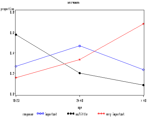
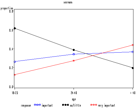
Figure 8.1 on page 140.
proc sort data = table8_1;
  by sex age;
run;
proc freq data = table8_1;
  weight frequency;
  by sex age;
  tables response/list ;
  ods output onewayfreqs = list;
run;
data list;
  set list;
  proportion = percent/100;
run;
goptions reset = all;
symbol1 i = join v=circle c=blue;
symbol2 i = join v=dot c=black;
symbol3 i = join v = star c = red;
axis1 order = (0 to .8 by .2) minor = none label=('proportion');
proc gplot data = list;
  by sex;
  plot proportion*age = response /vaxis = axis1;
run;
quit;


Table 8.2 on page 141.
data table8_1a;
  set table8_1;
  x1 = (sex ='men');
  x2 = (age = '24-40');
  x3 = (age = '> 40');
run;
proc logistic data = table8_1a ;
  freq frequency;
  class response (ref='no/little');
  model response = x1 x2 x3 /link=glogit ;
run;
          Response Profile
 Ordered                              Total
   Value     response             Frequency
       1     important                   94
       2     no/little                  105
       3     very important             101
Logits modeled use response='no/little' as the reference category.

         Model Fit Statistics
                              Intercept
               Intercept         and
Criterion        Only        Covariates
AIC              662.544        596.702
SC               669.952        626.332
-2 Log L         658.544        580.702
        Testing Global Null Hypothesis: BETA=0
Test                 Chi-Square       DF     Pr > ChiSq
Likelihood Ratio        77.8419        6         <.0001
Score                   74.9761        6         <.0001
Wald                    62.9703        6         <.0001

       Type III Analysis of Effects
                        Wald
Effect      DF    Chi-Square    Pr > ChiSq
x1           2        6.4173        0.0404
x2           2       17.5366        0.0002
x3           2       47.5933        <.0001

                   Analysis of Maximum Likelihood Estimates
                                             Standard         Wald
Parameter   response         DF   Estimate      Error   Chi-Square   Pr > ChiSq
Intercept   important         1    -0.5908     0.2840       4.3286       0.0375
Intercept   very important    1    -1.0391     0.3305       9.8843       0.0017
x1          important         1    -0.3881     0.3005       1.6677       0.1966
x1          very important    1    -0.8129     0.3210       6.4122       0.0113
x2          important         1     1.1283     0.3416      10.9059       0.0010
x2          very important    1     1.4780     0.4009      13.5912       0.0002
x3          important         1     1.5876     0.4029      15.5270       <.0001
x3          very important    1     2.9165     0.4229      47.5594       <.0001

                    Odds Ratio Estimates
                               Point          95% Wald
Effect    response          Estimate      Confidence Limits
x1        important            0.678       0.376       1.223
x1        very important       0.444       0.236       0.832
x2        important            3.090       1.582       6.037
x2        very important       4.384       1.998       9.620
x3        important            4.892       2.221      10.775
x3        very important      18.477       8.066      42.327
Table 8.3 on page 142.
proc sql;
  create table table8_1b as
  select *, sum(frequency) as total
  from table8_1a
  group by sex, age;
quit;
proc logistic data = table8_1b ;
  freq frequency;
  class response (ref='no/little');
  model response = x1 x2 x3 /link=glogit ;
  output out = table8_3 p=p ;
run;
data table8_3;
  set table8_3;
  fitted = p*total;
  pres = (frequency-fitted)/sqrt(fitted);
  if response=_level_;
run;
proc sort data = table8_3 ;
run;
proc print data = table8_3;
var sex age response frequency p fitted pres;
run;
Obs     sex      age     response          frequency       p        fitted      pres
  1    men      18-23    no/little             40       0.65246    42.4102    -0.37010
  2    men      18-23    important             17       0.24515    15.9346     0.26690
  3    men      18-23    very important         8       0.10239     6.6552     0.52128
  4    men      24-40    important             15       0.40753    17.9312    -0.69220
  5    men      24-40    very important        12       0.24149    10.6254     0.42171
  6    men      24-40    no/little             17       0.35099    15.4435     0.39608
  7    men      > 40     important             15       0.32034    13.1340     0.51489
  8    men      > 40     very important        18       0.50537    20.7201    -0.59756
  9    men      > 40     no/little              8       0.17429     7.1460     0.31948
 10    women    18-23    very important         7       0.18546     8.3455    -0.46576
 11    women    18-23    important             12       0.29034    13.0654    -0.29475
 12    women    18-23    no/little             26       0.52420    23.5891     0.49639
 13    women    24-40    very important        15       0.36388    16.3747    -0.33971
 14    women    24-40    important             21       0.40153    18.0687     0.68959
 15    women    24-40    no/little              9       0.23459    10.5566    -0.47908
 16    women    > 40     no/little              5       0.09759     5.8557    -0.35361
 17    women    > 40     very important        41       0.63798    38.2788     0.43983
 18    women    > 40     important             14       0.26443    15.8655    -0.46836
Table 8.4 on page 148.
data table8_1c;
  set table8_1a;
  if response = 'no/little' then resnum = 1;
  if response = 'important' then resnum = 2;
  if response = 'very important' then resnum = 3;
run;
proc logistic data = table8_1c descending ;
  freq frequency;
  model resnum = x1 x2 x3 /scale = none aggregate;
run;
Score Test for the Proportional Odds Assumption
Chi-Square       DF     Pr > ChiSq
    0.7139        3         0.8699

       Deviance and Pearson Goodness-of-Fit Statistics
Criterion        DF          Value     Value/DF     Pr > ChiSq
Deviance          7         4.5321       0.6474         0.7169
Pearson           7         4.5641       0.6520         0.7130
Number of unique profiles: 6

        Testing Global Null Hypothesis: BETA=0
Test                 Chi-Square       DF     Pr > ChiSq
Likelihood Ratio        77.2485        3         <.0001
Score                   70.0452        3         <.0001
Wald                    68.0278        3         <.0001

              Analysis of Maximum Likelihood Estimates
                                 Standard          Wald
Parameter      DF    Estimate       Error    Chi-Square    Pr > ChiSq
Intercept 3     1     -1.6546      0.2536       42.5742        <.0001
Intercept 2     1     -0.0433      0.2303        0.0354        0.8508
x1              1     -0.5762      0.2261        6.4936        0.0108
x2              1      1.1468      0.2773       17.1079        <.0001
x3              1      2.2322      0.2904       59.0806        <.0001

           Odds Ratio Estimates
             Point          95% Wald
Effect    Estimate      Confidence Limits
x1           0.562       0.361       0.875
x2           3.148       1.828       5.421
x3           9.320       5.275      16.467
