Note: This page has been updated using SAS 9.2 in January 2011.
Showing proc contents for the data file.
proc contents data=imm10 pos;
run;
And here are the results.
 # Variable Type Len Pos Label
-----------------------------------------------------------------------------------------------
15 cstr     Num    8 112
 5 homework Num    8  32 Time spent on math homework each week
11 math     Num    8  80 Math score
 4 meanses  Num    8  24 Mean SES for the school
 7 parented Num    8  48 Parents highest education level
10 percmin  Num    8  72 Percent minority in school
 8 public   Num    8  56 Public school: 1=public, 0=non-public
13 race     Num    8  96 race of student, 1=asian, 2=Hispanic, 3=Black, 4=White, 5=Native American
 9 ratio    Num    8  64 Student-Teacher ratio
18 region   Num    8 136
 1 schid    Num    8   0 School ID
19 schnum   Num    8 144 group(schid)
16 scsize   Num    8 120
14 sctype   Num    8 104 Type of school, 1=public, 2=catholic, 3=Private
                         other religious, 4=Private non-r
 3 ses      Num    8  16 Socioecnonomic Status
12 sex      Num    8  88 Sex: 1=male, 2=female
 2 stuid    Num    8   8 Student ID
17 urban    Num    8 128
 6 white    Num    8  40 Race: 1=white, 0=non-white
Page 48, Table 3.3
proc mixed data=imm10 covtest method=ml;
  class schid;
  model math = homework / solution ;
  random intercept homework / subject=schid type=un;
run;

                  Covariance Parameter Estimates

                                    Standard         Z
Cov Parm     Subject    Estimate       Error     Value        Pr Z

UN(1,1)      schid       61.8012     29.8685      2.07      0.0193
UN(2,1)      schid      -28.2571     15.4829     -1.83      0.0680
UN(2,2)      schid       19.9766      9.8069      2.04      0.0208
Residual                 43.0671      3.9292     10.96      <.0001

           Fit Statistics

-2 Log Likelihood              1769.4
AIC (smaller is better)        1781.4
AICC (smaller is better)       1781.7
BIC (smaller is better)        1783.2


  Null Model Likelihood Ratio Test

    DF    Chi-Square      Pr > ChiSq

     3        146.97          <.0001

                   Solution for Fixed Effects

                         Standard
Effect       Estimate       Error      DF    t Value    Pr > |t|

Intercept     44.7726      2.6031       9      17.20      <.0001
homework       2.0487      1.4722       9       1.39      0.1975
Page 50, table 3.4 equations.
proc mixed data=imm10 covtest method=ml;
  class schid;
  model math = homework public / solution ;
  random intercept homework / subject=schid type=un;
run;

                  Covariance Parameter Estimates

                                    Standard         Z
Cov Parm     Subject    Estimate       Error     Value        Pr Z

UN(1,1)      schid       40.6657     20.6116      1.97      0.0243
UN(2,1)      schid      -29.1507     14.4739     -2.01      0.0440
UN(2,2)      schid       21.6760     10.5313      2.06      0.0198
Residual                 42.9550      3.9104     10.98      <.0001

           Fit Statistics

-2 Log Likelihood              1750.8
AIC (smaller is better)        1764.8
AICC (smaller is better)       1765.3
BIC (smaller is better)        1767.0


  Null Model Likelihood Ratio Test

    DF    Chi-Square      Pr > ChiSq

     3         95.17          <.0001


                   Solution for Fixed Effects

                         Standard
Effect       Estimate       Error      DF    t Value    Pr > |t|

Intercept     58.0556      2.6944       8      21.55      <.0001
homework       1.9409      1.5247       9       1.27      0.2349
public       -14.6511      1.8315     240      -8.00      <.0001
Page 51, table 3.5 equations.
proc mixed data=imm10 covtest method=ml;
  class schid;
  model math = homework public homework*public / solution ;
  random intercept homework / subject=schid type=un;
run;
Results shown below. Note the interaction is positive but the bottom of page 50 shows the interaction is negative. We think this may be a typographical error.
                    Covariance Parameter Estimates

                                    Standard         Z
Cov Parm     Subject    Estimate       Error     Value        Pr Z

UN(1,1)      schid       40.4919     20.5363      1.97      0.0243
UN(2,1)      schid      -29.0135     14.4220     -2.01      0.0442
UN(2,2)      schid       21.5703     10.4935      2.06      0.0199
Residual                 42.9549      3.9104     10.98      <.0001

           Fit Statistics

-2 Log Likelihood              1750.8
AIC (smaller is better)        1766.8
AICC (smaller is better)       1767.4
BIC (smaller is better)        1769.2


  Null Model Likelihood Ratio Test

    DF    Chi-Square      Pr > ChiSq

     3         92.27          <.0001


                      Solution for Fixed Effects

                               Standard
Effect             Estimate       Error      DF    t Value    Pr > |t|

Intercept           59.2102      6.5967       8       8.98      <.0001
homework             1.0946      4.6679       8       0.23      0.8205
public             -15.9419      6.9767     240      -2.29      0.0232
homework*public      0.9473      4.9375     240       0.19      0.8480
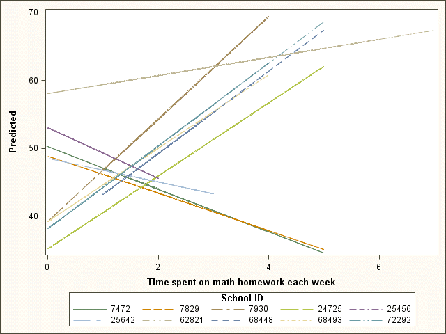
Page 52, Table 3.6 and Figure 3.8
proc mixed data= imm10 method=ml;
 class schid;
 model math = homework / solution outp=t;
 random intercept homework / subject=schid type=un g solution;
 ods output solutionR=randest;
run;
DATA randest2;
 set randest;
 by schid;
 retain intercept slope;
 if effect="Intercept" then  intercept = 44.772 + estimate;
 if effect="homework"  then  slope     = 2.0487 + estimate;
 if last.schid;
 keep schid intercept slope;
run;
proc print data=randest2 noobs;
 var intercept slope;
run;
intercept      slope

 50.2702     -3.14337
 48.8855     -2.75398
 39.1947      7.56630
 35.1560      5.39411
 53.0804     -3.73816
 48.5853     -1.76515
 58.0548      1.33518
 37.1518      6.05997
 39.1691      5.43043
 38.1722      6.10167
proc sgplot data = t;
  series x = homework y = pred /group=schid;
run;

Page 53, Figure 3.8

