
In this chapter, the data set is popular.
Table 4.1
Part 1: The variable sex is a fixed effect, not centered.
proc mixed data = pop ;
  model popular = sex/solution;
  random intercept / subject = school type = un;
run;
The Mixed Procedure

 Covariance Parameter Estimates
Cov Parm     Subject    Estimate
UN(1,1)      SCHOOL       0.8622
Residual                  0.4599

           Fit Statistics
-2 Res Log Likelihood          4492.9
AIC (smaller is better)        4496.9
AICC (smaller is better)       4496.9
BIC (smaller is better)        4502.1

  Null Model Likelihood Ratio Test
    DF    Chi-Square      Pr > ChiSq
     1       1728.72          <.0001

                   Solution for Fixed Effects
                         Standard
Effect       Estimate       Error      DF    t Value    Pr > |t|
Intercept      4.8972     0.09530      99      51.39      <.0001
SEX            0.8437     0.03096    1899      27.25      <.0001
Part 2: The variable sex is a fixed effect, raw centered. We first created
a centered variable csex for sex.
proc means data = pop mean ;
var sex;
run;

Analysis Variable : SEX pupil sex
        Mean
------------
   0.4870000
------------
data popc;
  set pop;
  csex = sex - .487;
run;
proc mixed data = popc ;
  model popular = csex/solution;
  random intercept / subject = school type = un;
run;
The Mixed Procedure
                   Covariance Parameter Estimates
Cov Parm     Subject    Estimate
UN(1,1)      SCHOOL       0.8622
Residual                  0.4599

           Fit Statistics
-2 Res Log Likelihood          4492.9
AIC (smaller is better)        4496.9
AICC (smaller is better)       4496.9
BIC (smaller is better)        4502.1

  Null Model Likelihood Ratio Test
    DF    Chi-Square      Pr > ChiSq
     1       1728.72          <.0001

                   Solution for Fixed Effects
                         Standard
Effect       Estimate       Error      DF    t Value    Pr > |t|
Intercept      5.3081     0.09410      99      56.41      <.0001
csex           0.8437     0.03096    1899      27.25      <.0001
Part 3: The variable sex is included as a random effect.
proc mixed data = pop ;
  model popular = sex/solution;
  random intercept sex/ subject = school type = un;
run;
Covariance Parameter Estimates
Cov Parm     Subject    Estimate
UN(1,1)      SCHOOL       0.9402
UN(2,1)      SCHOOL      -0.1410
UN(2,2)      SCHOOL       0.2725
Residual                  0.3924

           Fit Statistics
-2 Res Log Likelihood          4336.3
AIC (smaller is better)        4344.3
AICC (smaller is better)       4344.3
BIC (smaller is better)        4354.7

  Null Model Likelihood Ratio Test
    DF    Chi-Square      Pr > ChiSq
     3       1885.30          <.0001

                   Solution for Fixed Effects
                         Standard
Effect       Estimate       Error      DF    t Value    Pr > |t|
Intercept      4.8901     0.09901      99      49.39      <.0001
SEX            0.8431     0.05963      99      14.14      <.0001
Part 4: The variable sex is centered and is a random effect.
proc mixed data = popc ;
  model popular = csex/solution;
  random intercept csex/ subject = school type = un;
run;
Covariance Parameter Estimates
Cov Parm     Subject    Estimate
UN(1,1)      SCHOOL       0.8675
UN(2,1)      SCHOOL     -0.00825
UN(2,2)      SCHOOL       0.2725
Residual                  0.3924

           Fit Statistics
-2 Res Log Likelihood          4336.3
AIC (smaller is better)        4344.3
AICC (smaller is better)       4344.3
BIC (smaller is better)        4354.7

  Null Model Likelihood Ratio Test
    DF    Chi-Square      Pr > ChiSq
     3       1885.30          <.0001

                   Solution for Fixed Effects
                         Standard
Effect       Estimate       Error      DF    t Value    Pr > |t|
Intercept      5.3007     0.09424      99      56.25      <.0001
csex           0.8431     0.05963      99      14.14      <.0001
Table 4.2 on page 60.
Part 1: No interaction, no centering.
proc mixed data = pop ;
  model popular = sex texp /solution;
  random intercept sex/ subject = school type = un;
run;
 Covariance Parameter Estimates
Cov Parm     Subject    Estimate
UN(1,1)      SCHOOL       0.4116
UN(2,1)      SCHOOL      0.02089
UN(2,2)      SCHOOL       0.2733
Residual                  0.3925

           Fit Statistics
-2 Res Log Likelihood          4275.9
AIC (smaller is better)        4283.9
AICC (smaller is better)       4283.9
BIC (smaller is better)        4294.3

                   Solution for Fixed Effects
                         Standard
Effect       Estimate       Error      DF    t Value    Pr > |t|
Intercept      3.3400      0.1608      98      20.77      <.0001
SEX            0.8431     0.05969      99      14.13      <.0001
TEXP           0.1084     0.01022    1800      10.61      <.0001
Part 2: With interaction, but no centering.
data pop1;
  set pop;
  genxexp = sex*texp;
run;
proc mixed data = pop1 ;
  model popular = sex texp genxexp/solution;
  random intercept sex /subject = school type=un ;
run;
Covariance Parameter Estimates
Cov Parm     Subject    Estimate
UN(1,1)      SCHOOL       0.4120
UN(2,1)      SCHOOL      0.02343
UN(2,2)      SCHOOL       0.2264
Residual                  0.3924

           Fit Statistics
-2 Res Log Likelihood          4268.4
AIC (smaller is better)        4276.4
AICC (smaller is better)       4276.5
BIC (smaller is better)        4286.9

                   Solution for Fixed Effects
                         Standard
Effect       Estimate       Error      DF    t Value    Pr > |t|
Intercept      3.3135      0.1610      98      20.58      <.0001
SEX            1.3296      0.1330      98       9.99      <.0001
TEXP           0.1102     0.01023    1800      10.77      <.0001
genxexp      -0.03403    0.008457    1800      -4.02      <.0001
Part 3: Centering, but no interaction. We first created new variables
csex and ctexp and their interaction term.
proc means data = pop mean;
var sex texp;
run;

The MEANS Procedure
Variable    Label                                  Mean
-------------------------------------------------------
SEX         pupil sex                         0.4870000
TEXP        teacher experience in years      14.2630000
-------------------------------------------------------

data pop2;
  set pop;
  csex = sex - 0.487;
  ctexp = texp - 14.263;
  cx = csex*ctexp;
run;
proc mixed data = pop2 ;
  model popular = csex ctexp /solution;
  random intercept csex /subject = school type=un ;
run;
Covariance Parameter Estimates
Cov Parm     Subject    Estimate
UN(1,1)      SCHOOL       0.4967
UN(2,1)      SCHOOL       0.1540
UN(2,2)      SCHOOL       0.2733
Residual                  0.3925

           Fit Statistics
-2 Res Log Likelihood          4275.9
AIC (smaller is better)        4283.9
AICC (smaller is better)       4283.9
BIC (smaller is better)        4294.3

                   Solution for Fixed Effects
                         Standard
Effect       Estimate       Error      DF    t Value    Pr > |t|
Intercept      5.2960     0.07192      98      73.63      <.0001
csex           0.8431     0.05969      99      14.13      <.0001
ctexp          0.1084     0.01022    1800      10.61      <.0001
Part 4: Centering and with interaction.
proc mixed data = pop2 ;
  model popular = csex ctexp cx/solution;
  random intercept csex /subject = school type=un ;
run;
Covariance Parameter Estimates
Cov Parm     Subject    Estimate
UN(1,1)      SCHOOL       0.4885
UN(2,1)      SCHOOL       0.1337
UN(2,2)      SCHOOL       0.2264
Residual                  0.3924

           Fit Statistics
-2 Res Log Likelihood          4268.4
AIC (smaller is better)        4276.4
AICC (smaller is better)       4276.5
BIC (smaller is better)        4286.9

                   Solution for Fixed Effects
                         Standard
Effect       Estimate       Error      DF    t Value    Pr > |t|
Intercept      5.2969     0.07135      98      74.24      <.0001
csex           0.8442     0.05562      98      15.18      <.0001
ctexp         0.09366     0.01085    1800       8.63      <.0001
cx           -0.03403    0.008457    1800      -4.02      <.0001
Figure 4.3. Regression lines for popularity of girls and boys,
predicted by teacher experience, texp.
This uses model in Part 2 of Table 4.2. We will have to
manually create the predicted values by the fixed part of the model.
data fig4_3;
  set pop1;
  pred =  3.3135 + 1.3296* sex +  0.1102*texp  -0.03403*genxexp;
run;

axis1 order = (0 to 30 by 10) minor = none label = (" ");
axis2 order = (3.5 to 7 by .5) minor = none label = (" ");
symbol i = join;
proc gplot data = fig4_3;
  plot pred*texp = sex /vaxis =axis2 haxis=axis1;
run;
quit;
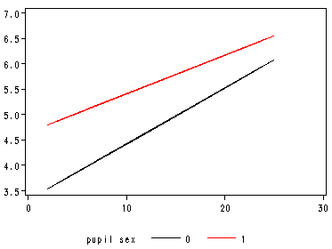
Table 4.3
Part 1: Intercept only.
This has been done in Chapter 2, Table 2.1.
Part 2: The variable sex is included as a fixed effect.
This has been done in Table 4.1.
Part 3: The variable texp is also included.
proc mixed data = pop1 ;
  model popular = sex texp  / outp = test solution;
  random intercept  /subject = school type=un ;
run;
Covariance Parameter Estimates
Cov Parm     Subject    Estimate
UN(1,1)      SCHOOL       0.4860
Residual                  0.4599

           Fit Statistics
-2 Res Log Likelihood          4444.4
AIC (smaller is better)        4448.4
AICC (smaller is better)       4448.4
BIC (smaller is better)        4453.6

                   Solution for Fixed Effects
                         Standard
Effect       Estimate       Error      DF    t Value    Pr > |t|
Intercept      3.5607      0.1715      98      20.76      <.0001
SEX            0.8447     0.03095    1899      27.29      <.0001
TEXP          0.09345     0.01085    1899       8.61      <.0001
Part 4: This has been done in Table 4.2.
Part 5: This is done in Table 4.2.
Table 4.4 can be produced manually based on the equations provided in
this section. We omit the calculation here.