Page 271 Figure 12.1 Logistic function for the depression data set.
NOTE: We were unable to reproduce this graph.
Page 273 Table 12.1 Classification of individuals by depression level and sex.
data depress;
set "c:\pma5\depress";
run;
proc freq data = depress;
tables sex*cases;
run;

The FREQ Procedure

Table of SEX by CASES

SEX       CASES

Frequency|
Percent  |
Row Pct  |
Col Pct  |       0|       1|  Total
---------+--------+--------+
       1 |    101 |     10 |    111
         |  34.35 |   3.40 |  37.76
         |  90.99 |   9.01 |
         |  41.39 |  20.00 |
---------+--------+--------+
       2 |    143 |     40 |    183
         |  48.64 |  13.61 |  62.24
         |  78.14 |  21.86 |
         |  58.61 |  80.00 |
---------+--------+--------+
Total         244       50      294
            82.99    17.01   100.00
Page 274 Odds ratios and coefficients
data depress;
set depress;
sex1 = sex - 1;
run;

proc logistic data = depress desc;
model cases = sex1;
run;

The LOGISTIC Procedure

             Analysis of Maximum Likelihood Estimates

                               Standard          Wald
Parameter    DF    Estimate       Error    Chi-Square    Pr > ChiSq

Intercept     1     -2.3125      0.3315       48.6603        <.0001
sex1          1      1.0385      0.3767        7.6013        0.0058

           Odds Ratio Estimates

             Point          95% Wald
Effect    Estimate      Confidence Limits

sex1         2.825       1.350       5.911
(some output omitted)
Page 275 The coefficients at the bottom of the page.
proc logistic data = depress desc;
model cases = age income;
run;

The LOGISTIC Procedure

             Analysis of Maximum Likelihood Estimates

                               Standard          Wald
Parameter    DF    Estimate       Error    Chi-Square    Pr > ChiSq

Intercept     1      0.0280      0.4872        0.0033        0.9542
AGE           1     -0.0202     0.00890        5.1385        0.0234
INCOME        1     -0.0413      0.0141        8.6500        0.0033
(some output omitted)
Page 276 These numbers are obtained from the output from page 275.
Page 278 Table at the top of the page
NOTE: We will create the interaction of the two dummy variables (which we called dincemp) in this data step for use in the example on page 279.
data depress;
set depress;
if income >= 10 then duminc = 0;
else duminc = 1;
if employ = 2 or employ = 3 then dumemp = 1;
else dumemp = 0;
if employ = 7 then dumemp = .;
dincemp = duminc*dumemp;
run;

proc logistic data = depress desc;
model cases = duminc dumemp;
run;
quit;


The LOGISTIC Procedure
             Analysis of Maximum Likelihood Estimates
                               Standard          Wald
Parameter    DF    Estimate       Error    Chi-Square    Pr > ChiSq
Intercept     1     -1.9345      0.2259       73.3313        <.0001
duminc        1      0.2723      0.3377        0.6502        0.4200
dumemp        1      1.0285      0.3487        8.6990        0.0032


           Odds Ratio Estimates
             Point          95% Wald
Effect    Estimate      Confidence Limits
duminc       1.313       0.677       2.545
dumemp       2.797       1.412       5.540
(some output omitted)
Page 279 middle of the page
proc logistic data = depress desc;
model cases = duminc dumemp dincemp;
run;
quit;

        Testing Global Null Hypothesis: BETA=0
Test                 Chi-Square       DF     Pr > ChiSq
Likelihood Ratio        16.8347        3         0.0008
Score                   22.4086        3         <.0001
Wald                    16.8136        3         0.0008

        Testing Global Null Hypothesis: BETA=0
Test                 Chi-Square       DF     Pr > ChiSq
Likelihood Ratio         8.6045        2         0.0135
Score                    9.5814        2         0.0083
Wald                     9.0619        2         0.0108


The LOGISTIC Procedure

             Analysis of Maximum Likelihood Estimates
                               Standard          Wald
Parameter    DF    Estimate       Error    Chi-Square    Pr > ChiSq
Intercept     1     -1.7346      0.2214       61.3804        <.0001
duminc        1     -0.3756      0.4349        0.7458        0.3878
dumemp        1      0.3175      0.4520        0.4935        0.4824
dincemp       1      2.1981      0.7888        7.7651        0.0053


           Odds Ratio Estimates
              Point          95% Wald
Effect     Estimate      Confidence Limits
duminc        0.687       0.293       1.611
dumemp        1.374       0.566       3.332
dincemp       9.008       1.919      42.276
(some output omitted)
Page 280 bottom of the page
NOTE: The likelihood ratio chi-square values needed are given in the output for the two models shown above: 16.83-8.6 = 8.23.
Page 287 middle of the page
data depress;
set depress;
if age < 28 then age0 = 1;
else age0 = 0;
if age >=28 & age <= 42 then age1 = 1;
else age1 = 0;
if age >=43 & age <= 58 then age2 = 1;
else age2 = 0;
if age >=59 & age <= 89 then age3 = 1;
else age3 = 0;
run;

proc logistic data = depress desc;
model cases = age1 age2 age3 income sex;
run;
quit;

The LOGISTIC Procedure

             Analysis of Maximum Likelihood Estimates
                               Standard          Wald
Parameter    DF    Estimate       Error    Chi-Square    Pr > ChiSq
Intercept     1     -2.1595      0.7830        7.6056        0.0058
age1          1      0.0747      0.4318        0.0299        0.8626
age2          1     -0.5706      0.4744        1.4468        0.2290
age3          1     -0.8853      0.4563        3.7643        0.0524
income        1     -0.0380      0.0149        6.5298        0.0106
sex           1      0.9238      0.3864        5.7147        0.0168
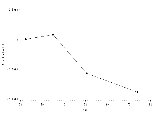
Page 289 Figure 12.2 Estimated coefficients for age quartiles by midpoint of the quartile
NOTE: We need to use ODS to capture the coefficients in a data set. We use the ods trace on and ods trace off statements so that SAS prints the names of the various tables in the log. Then we can look there to get the name of the table that we need to include on the ods output statement. The print procedures are not necessary; they just help see what the data sets look like before the next addition or modification.
ods trace on;
proc logistic data = depress desc;
model cases = age1 age2 age3 income sex;
ods output ParameterEstimates = parms1;
run;
quit;
ods trace off;

proc print data = parms1;
run;

data parms1;
if _n_ = 1 then do;
variable = "age0";
estimate = 0;
end;
output;
set parms1;
run;

data parms;
set parms1;
if variable = "age0" then newage = 22.5;
if variable = "age1" then newage = 35;
if variable = "age2" then newage = 50.5;
if variable = "age3" then newage = 74;
if variable in("age0" "age1" "age2" "age3");
run;

proc print data = parms;
run;

axis1 label=(a=90 'Coefficient b') order = (-1 to .5 by .5);
axis2 label=("Age") order = (20 to 80 by 10);
symbol1 i=join v=dot;
proc gplot data = parms;
plot estimate*newage / vaxis=axis1 haxis = axis2;
run;
quit;
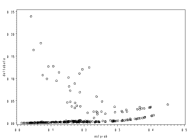
Page 291 Figure 12.3 Delta beta measures to assess the influence of individual patterns on estimated coefficients
NOTE: We are including the difchisq (delta chi-square) statistic here for use on page 294.
proc logistic data = depress desc;
model cases = sex income age;
output out=pred p=estprob c=deltabeta DIFCHISQ=deltachi;
run;
quit;

symbol1 i=none v=circle ;
axis1 order=(0 to .5 by .1) ;
axis2 label=(angle=90) order=(0 to .25 by .05);
proc gplot data=pred;
plot deltabeta*estprob / haxis=axis1 vaxis=axis2;
run;
quit;
Page 292 Table 12.2 Percent change in estimated parameters when including and excluding influential patterns
*line 1 of table;

proc logistic data = depress desc;
model cases = age income sex;
run;
quit;

The LOGISTIC Procedure
             Analysis of Maximum Likelihood Estimates
                               Standard          Wald
Parameter    DF    Estimate       Error    Chi-Square    Pr > ChiSq
Intercept     1     -1.6059      0.8465        3.5987        0.0578
age           1     -0.0210     0.00904        5.3744        0.0204
income        1     -0.0366      0.0141        6.7343        0.0095
sex           1      0.9294      0.3858        5.8032        0.0160

proc sort data = pred1;
by deltabeta;
run;

proc print data = pred1(firstobs=292);
var id deltabeta;
run;

Obs     id    deltabeta

292    288     0.16373
293     99     0.17896
294     68     0.23899


data pred1;
set pred;
x = 0;
if deltabeta > .1637310 then x = 3;
if deltabeta > .1789604 then x = 2;
if deltabeta > .2084397 then x = 1;
run;

proc print data = pred1;
var x deltabeta;
where x ne 0;
run;

Obs    x    deltabeta

292    3     0.16373
293    2     0.17896
294    1     0.23899

* line 2 of table;

proc logistic data = pred1 desc;
model cases = age income sex;
where x ne 1;
run;
quit;

The LOGISTIC Procedure

             Analysis of Maximum Likelihood Estimates
                               Standard          Wald
Parameter    DF    Estimate       Error    Chi-Square    Pr > ChiSq
Intercept     1     -1.6991      0.8737        3.7818        0.0518
age           1     -0.0215     0.00912        5.5826        0.0181
income        1     -0.0421      0.0150        7.8971        0.0050
sex           1      1.0301      0.4008        6.6050        0.0102


* line 3 of table;

proc logistic data = pred1 desc;
model cases = age income sex;
where x ne 2;
run;
quit;

The LOGISTIC Procedure
             Analysis of Maximum Likelihood Estimates
                               Standard          Wald
Parameter    DF    Estimate       Error    Chi-Square    Pr > ChiSq
Intercept     1     -1.7570      0.8712        4.0674        0.0437
age           1     -0.0234     0.00925        6.4023        0.0114
income        1     -0.0358      0.0142        6.3918        0.0115
sex           1      1.0505      0.4008        6.8707        0.0088


* line 4 of table;

proc logistic data = pred1 desc;
model cases = age income sex;
where x ne 3;
run;
quit;

The LOGISTIC Procedure
             Analysis of Maximum Likelihood Estimates
                               Standard          Wald
Parameter    DF    Estimate       Error    Chi-Square    Pr > ChiSq
Intercept     1     -1.7138      0.8721        3.8619        0.0494
age           1     -0.0229     0.00920        6.1894        0.0129
income        1     -0.0389      0.0145        7.1596        0.0075
sex           1      1.0419      0.4009        6.7562        0.0093

* line 5 of table;

proc logistic data = pred1 desc;
model cases = age income sex;
where x = 0;
run;
quit;

The LOGISTIC Procedure
             Analysis of Maximum Likelihood Estimates
                               Standard          Wald
Parameter    DF    Estimate       Error    Chi-Square    Pr > ChiSq
Intercept     1     -2.0252      0.9419        4.6233        0.0315
age           1     -0.0263     0.00953        7.6125        0.0058
income        1     -0.0443      0.0156        8.0351        0.0046
sex           1      1.3094      0.4407        8.8267        0.0030
Page 293 Table 12.3 Estimated probability of being a case (p-hat) for five influential observations
proc print data = pred1 noobs round;
var id age income sex cases estprob;
where id = 288 or id = 99 or id = 143 or id = 232 or id = 68;
run;

143     40      45       1       0        0.04
232     40      45       1       0        0.04
288     61      28       1       1        0.05
 99     72      11       1       1        0.07
 68     40      45       1       1        0.04
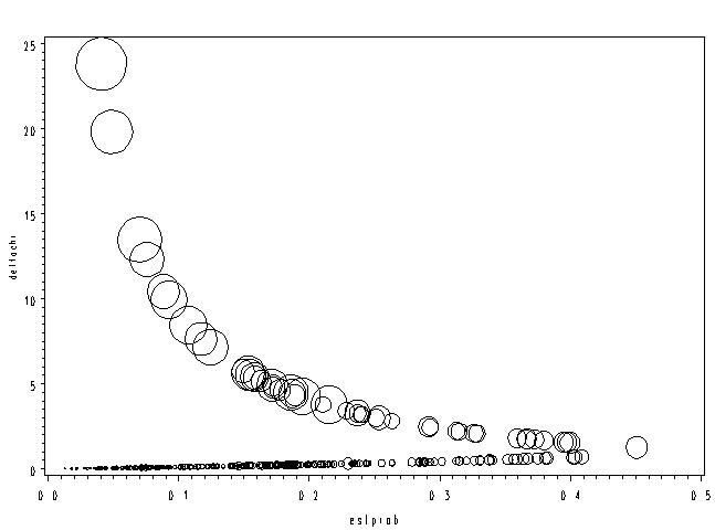
Page 294 Figure 12.4 Delta chi-square measure to assess influence of pattern on overall fit with symbol size proportional to delta beta
NOTE: This graph looks slightly different from the graph in the text. This is probably because SAS and Stata calculate the covariate patterns in different ways.
symbol1 color=black interpol=r value=circle height=1;
axis1 order=(0 to 25 by 5) label=(angle=90 color=black height=0.75);
axis2 order=(0 to .5 by .1);
proc gplot data=pred;
bubble deltachi*estprob=deltabeta / bsize=20 haxis=axis2 vaxis=axis1;
run;
quit;
Page 296 Figure 12.5 Percentage of individuals correctly classified by logistic regression.
NOTE: We were unable to reproduce this graph.
Page 297 Figure 12.6 ROC curve from logistic regression for the depression data set.
NOTE: We were unable to reproduce this graph.