Version info: Code for this page was tested in SAS 9.3.
For this chapter, you will need to use the syntax provided in Appendix A to access the School and Mice datasets.
Figure 18.2, page 466 is not reproduced.
Table 18.2, page 468 Estimated coefficients from three naive linear regression models ignoring the hierarchical structure of the school data. Note that for Model 3, we believe there is a typo where the coefficient for “Three hours” was copied for “Four or more hours”.
PROC SORT data = School;
  by descending newSCHTYPE descending newHW;
RUN;

/* Table 18.2 */
PROC GLM data = School order = data;
  class newSCHTYPE;
  model MATH = newSCHTYPE / solution;
RUN;

The GLM Procedure
Dependent Variable: MATH
                                        Sum of
Source                      DF         Squares     Mean Square    F Value    Pr > F
Model                        1      7517.11179      7517.11179      74.89    <.0001 Error 517 51890.93446 100.36931 Corrected Total 518 59408.04624 R-Square Coeff Var Root MSE MATH Mean 0.126534 19.36960 10.01845 51.72254 Source DF Type I SS Mean Square F Value Pr > F
newSCHTYPE                   1     7517.111786     7517.111786      74.89    <.0001 Source DF Type III SS Mean Square F Value Pr > F
newSCHTYPE                   1     7517.111786     7517.111786      74.89    <.0001 Standard Parameter Estimate Error t Value Pr > |t|
Intercept         56.49009901 B      0.70489558      80.14      <.0001
newSCHTYPE 1      -7.80555642 B      0.90194247      -8.65      <.0001
newSCHTYPE 0       0.00000000 B       .                .         .

NOTE: The X'X matrix has been found to be singular, and a generalized inverse was used to solve
      the normal equations.  Terms whose estimates are followed by the letter 'B' are not
      uniquely estimable.


PROC GLM data = School order = data;
  class newSCHTYPE;
  model MATH = newSCHTYPE SES / solution;
RUN;

The GLM Procedure
Dependent Variable: MATH

                                        Sum of
Source                      DF         Squares     Mean Square    F Value    Pr > F
Model                        2     14923.96488      7461.98244      86.56    <.0001 Error 516 44484.08136 86.20946 Corrected Total 518 59408.04624 R-Square Coeff Var Root MSE MATH Mean 0.251211 17.95137 9.284905 51.72254 Source DF Type I SS Mean Square F Value Pr > F
newSCHTYPE                   1     7517.111786     7517.111786      87.20    <.0001
SES                          1     7406.853097     7406.853097      85.92    <.0001 Source DF Type III SS Mean Square F Value Pr > F
newSCHTYPE                   1      621.850871      621.850871       7.21    0.0075
SES                          1     7406.853097     7406.853097      85.92    <.0001 Standard Parameter Estimate Error t Value Pr > |t|
Intercept         53.37221655 B      0.73479649      72.64      <.0001
newSCHTYPE 1      -2.69017405 B      1.00164705      -2.69      0.0075
newSCHTYPE 0       0.00000000 B       .                .         .
SES                5.14426413        0.55498834       9.27      <.0001
NOTE: The X'X matrix has been found to be singular, and a generalized inverse was used to solve
      the normal equations.  Terms whose estimates are followed by the letter 'B' are not
      uniquely estimable.

PROC GLM data = School order = data;
  class newSCHTYPE newHW;
  model MATH = newSCHTYPE SES newHW / solution;
RUN;

The GLM Procedure
Dependent Variable: MATH
                                        Sum of
Source                      DF         Squares     Mean Square    F Value    Pr > F
Model                        7     20787.19803      2969.59972      39.29    <.0001 Error 511 38620.84821 75.57896 Corrected Total 518 59408.04624 R-Square Coeff Var Root MSE MATH Mean 0.349905 16.80818 8.693616 51.72254 Source DF Type I SS Mean Square F Value Pr > F
newSCHTYPE                   1     7517.111786     7517.111786      99.46    <.0001
SES                          1     7406.853097     7406.853097      98.00    <.0001
newHW                        5     5863.233151     1172.646630      15.52    <.0001 Source DF Type III SS Mean Square F Value Pr > F
newSCHTYPE                   1      215.042228      215.042228       2.85    0.0923
SES                          1     4888.876929     4888.876929      64.69    <.0001
newHW                        5     5863.233151     1172.646630      15.52    <.0001 Standard Parameter Estimate Error t Value Pr > |t|
Intercept         51.37485359 B      1.50805261      34.07      <.0001
newSCHTYPE 1      -1.60459840 B      0.95127248      -1.69      0.0923
newSCHTYPE 0       0.00000000 B       .                .         .
SES                4.27563995        0.53161476       8.04      <.0001
newHW      5       8.07390470 B      1.91180028       4.22      <.0001
newHW      4       7.56010333 B      1.88968358       4.00      <.0001
newHW      3       5.20851187 B      1.85282204       2.81      0.0051
newHW      2       0.22640909 B      1.57858349       0.14      0.8860
newHW      1      -1.39021887 B      1.46388306      -0.95      0.3427
newHW      0       0.00000000 B       .                .         .
NOTE: The X'X matrix has been found to be singular, and a generalized inverse was used to solve
      the normal equations.  Terms whose estimates are followed by the letter 'B' are not
      uniquely estimable.
Table 18.3, page 472 Estimated coefficients from three random slope regression models accounting for the hierarchical structure of the school data.
/* Table 18.3 */
PROC MIXED data = School order = data noclprint;
  class newSCHTYPE SCHOOL;
  model MATH = newSCHTYPE / solution;
  random Int / type = un sub=SCHOOL;
RUN;

The Mixed Procedure
                  Model Information
Data Set                     WORK.SCHOOL
Dependent Variable           MATH
Covariance Structure         Unstructured
Subject Effect               SCHOOL
Estimation Method            REML
Residual Variance Method     Profile
Fixed Effects SE Method      Model-Based
Degrees of Freedom Method    Containment

            Dimensions
Covariance Parameters             2
Columns in X                      3
Columns in Z Per Subject          1
Subjects                         23
Max Obs Per Subject              67

          Number of Observations
Number of Observations Read             519
Number of Observations Used             519
Number of Observations Not Used           0

                     Iteration History
Iteration    Evaluations    -2 Res Log Like       Criterion
        0              1      3861.02842646
        1              3      3789.18082462      0.00034325
        2              1      3788.60625480      0.00004068
        3              1      3788.54373285      0.00000078
        4              1      3788.54261121      0.00000000
                   Convergence criteria met.

 Covariance Parameter Estimates
Cov Parm     Subject    Estimate
UN(1,1)      SCHOOL      19.1533
Residual                 81.2337
           Fit Statistics
-2 Res Log Likelihood          3788.5
AIC (smaller is better)        3792.5
AICC (smaller is better)       3792.6
BIC (smaller is better)        3794.8

  Null Model Likelihood Ratio Test
    DF    Chi-Square      Pr > ChiSq
     1         72.49          <.0001 Solution for Fixed Effects new Standard Effect SCHTYPE Estimate Error DF t Value Pr > |t|
Intercept                 54.6684      1.7402      21      31.41      <.0001 newSCHTYPE 1 -5.9060 2.1369 496 -2.76 0.0059 newSCHTYPE 0 0 . . . . Type 3 Tests of Fixed Effects Num Den Effect DF DF F Value Pr > F
newSCHTYPE       1     496       7.64    0.0059


PROC MIXED data = School order = data noclprint;
  class newSCHTYPE SCHOOL;
  model MATH = newSCHTYPE SES / solution;
  random Int / type = un sub=SCHOOL;
RUN;

[some output ommitted]

 Covariance Parameter Estimates
Cov Parm     Subject    Estimate
UN(1,1)      SCHOOL      12.2516
Residual                 75.2895

           Fit Statistics
-2 Res Log Likelihood          3741.4
AIC (smaller is better)        3745.4
AICC (smaller is better)       3745.4
BIC (smaller is better)        3747.6

  Null Model Likelihood Ratio Test
    DF    Chi-Square      Pr > ChiSq
     1         39.39          <.0001 Solution for Fixed Effects new Standard Effect SCHTYPE Estimate Error DF t Value Pr > |t|
Intercept                 52.8099      1.4733      21      35.85      <.0001
newSCHTYPE    1           -2.4527      1.8448     495      -1.33      0.1843
newSCHTYPE    0                 0           .       .        .         .
SES                        4.1319      0.5869     495       7.04      <.0001 Type 3 Tests of Fixed Effects Num Den Effect DF DF F Value Pr > F
newSCHTYPE       1     495       1.77    0.1843
SES              1     495      49.56    <.0001

PROC MIXED data = School order = data noclprint;
  class newSCHTYPE newHW SCHOOL;
  model MATH = newSCHTYPE SES newHW / solution;
  random Int / type = un sub=SCHOOL;
RUN;

[some output ommitted]

  Covariance Parameter Estimates
Cov Parm     Subject    Estimate
UN(1,1)      SCHOOL      11.8628
Residual                 65.8440
           Fit Statistics
-2 Res Log Likelihood          3657.4
AIC (smaller is better)        3661.4
AICC (smaller is better)       3661.4
BIC (smaller is better)        3663.7

  Null Model Likelihood Ratio Test
    DF    Chi-Square      Pr > ChiSq
     1         38.62          <.0001 Solution for Fixed Effects new new Standard Effect SCHTYPE HW Estimate Error DF t Value Pr > |t|
Intercept                        50.9881      1.9106      21      26.69      <.0001
newSCHTYPE    1                  -1.6503      1.7931     490      -0.92      0.3578
newSCHTYPE    0                        0           .       .        .         .
SES                               3.4652      0.5578     490       6.21      <.0001
newHW                    5        7.7219      1.8686     490       4.13      <.0001
newHW                    4        7.6464      1.8339     490       4.17      <.0001 newHW 3 5.3106 1.8002 490 2.95 0.0033 newHW 2 0.7257 1.5419 490 0.47 0.6381 newHW 1 -1.2868 1.4251 490 -0.90 0.3670 newHW 0 0 . . . . Type 3 Tests of Fixed Effects Num Den Effect DF DF F Value Pr > F
newSCHTYPE       1     490       0.85    0.3578
SES              1     490      38.60    <.0001
newHW            5     490      15.45    <.0001
Figure 18.3 is not reproduced.
Table 18.4, page 480 is not reproduced. To create it, you can simply run models for all pairwise combination of variables.
Figure 18.4, page 483 Weight over time for 14 Mice.
/*Figure 18.4 page 483 */
symbol1 value = circle color = black interpol = join repeat = 14;
PROC GPLOT data = Mice;
  plot WEIGHT * DAY = ID / nolegend;
RUN;
QUIT;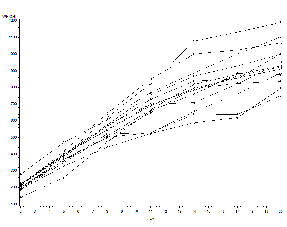
Table 18.5, page 485Estimates for random intercept and random slope models with different correlation structures. Note that these are complex random effects models to be fitting on only 14 mice. The parameter estimates vary between packages, with some reporting Errors or warnings in the optimization.
DATA Mice;
  set Mice;
  cDAY = DAY;
RUN;

PROC SORT data = Mice;
  by cDAY;
RUN;

/* Table 18.5, page 485*/
PROC MIXED data = Mice METHOD=ML noclprint;
  class ID cDay;
  model WEIGHT = DAY / solution;
  random int DAY / subject = ID;
  repeated cDAY /  subject = ID type = AR(1);
RUN;

The Mixed Procedure
                  Model Information
Data Set                     WORK.MICE
Dependent Variable           WEIGHT
Covariance Structures        Variance Components,
                             Autoregressive
Subject Effects              ID, ID
Estimation Method            ML
Residual Variance Method     Profile
Fixed Effects SE Method      Model-Based
Degrees of Freedom Method    Containment

            Dimensions
Covariance Parameters             4
Columns in X                      2
Columns in Z Per Subject          2
Subjects                         14
Max Obs Per Subject               7

          Number of Observations
Number of Observations Read              98
Number of Observations Used              98
Number of Observations Not Used           0

                     Iteration History
Iteration    Evaluations        -2 Log Like       Criterion
        0              1      1189.14416371
        1              3      1084.16542429      0.00090715
        2              2      1083.77544184      0.00005750
        3              1      1083.74783386      0.00000073
        4              1      1083.74749894      0.00000000
                   Convergence criteria met.

 Covariance Parameter Estimates
Cov Parm      Subject    Estimate
Intercept     ID                0
DAY           ID          25.7119
AR(1)         ID           0.7166
Residual                  5931.47

          Fit Statistics
-2 Log Likelihood              1083.7
AIC (smaller is better)        1093.7
AICC (smaller is better)       1094.4
BIC (smaller is better)        1096.9

                   Solution for Fixed Effects
                         Standard
Effect       Estimate       Error      DF    t Value    Pr > |t|
Intercept      156.82     22.0092      13       7.13      <.0001
DAY           41.0553      2.0202      13      20.32      <.0001 Type 3 Tests of Fixed Effects Num Den Effect DF DF F Value Pr > F
DAY             1      13     413.02    <.0001

PROC MIXED data = Mice METHOD=ML noclprint;
  class ID cDay;
  model WEIGHT = DAY / solution;
  random int DAY / subject = ID;
  repeated cDAY /  subject = ID type = cs;
RUN;

 Covariance Parameter Estimates
Cov Parm      Subject    Estimate
Intercept     ID                0
DAY           ID          50.4134
CS            ID          -533.47
Residual                  3734.32

           Fit Statistics
-2 Log Likelihood              1118.3
AIC (smaller is better)        1128.3
AICC (smaller is better)       1129.0
BIC (smaller is better)        1131.5

                   Solution for Fixed Effects
                         Standard
Effect       Estimate       Error      DF    t Value    Pr > |t|
Intercept      180.41     11.3171      13      15.94      <.0001
DAY           41.0544      2.1586      13      19.02      <.0001 Type 3 Tests of Fixed Effects Num Den Effect DF DF F Value Pr > F
DAY             1      13     361.73    <.0001